Transforming and analyzing data
Why use dplyr?
- Designed to work with data frames, which is what journalists are used to
- Great for data exploration and transformation
- Intuitive to write and easy to read, especially when using the “chaining” syntax of pipes
Five basic verbs
filter()select()arrange()mutate()summarize()plusgroup_by()
Our data
We’re going to be wrangling some pretty big data– murders over decades across the country.
This case-level data was acquired by the Murder Accountability Project from the Justice Department.
We’re going to use the basics of dplyr verb functions to analyze the data and see if there are any stories there might be worth pursuing.
Remember that huge SPSS data set we imported in the previous chapter?
I saved all that code we wrote to import it, renaming columns, and joining values and labels into an R script: import_murders.R. This is reproducibility in action.
Check out what it looks like– it’s about 100 lines of code long but only one line is required to run the script below.
Before running the command, make sure the script is in the working directory folder and that the SHR76_16.sav.zip file is in the data sub folder. For example, on my computer, the import_murders.R script is in the dplyr folder and SHR76_16.sav.zip file is in the dplyr/data folder.
This is going to take a few minutes to run.
source("import_murders.R")Alright, the import_murders.R script unzipped data, imported it, and transformed it into a workable dataframe and saved it to our environment as the object murders for us to analyze. You probably got some warnings in the console but that’s okay.
View(murders)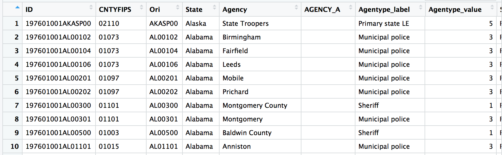
Here’s the data dictionary.
What are we dealing with here?
Number of rows (cases)?
nrow(murders)## [1] 752313How many municipalities?
We’ll use a couple base R functions: unique() and length().
# Make a list of cities based on the unique() function
how_many <- unique(murders$MSA_label)

# Count up how many are in the list
length(how_many)
## [1] 409Whew, let’s not overwhelm ourselves with all this data as we’re getting started out.
When I get a new data set I like to see what it’s made of. So I can begin to get a sense of how to summarize it or take it apart.
Start with the glimpse() function from dplyr– it will give a brief look at the variables in the data set and the data type.
glimpse(murders)## Observations: 752,313
## Variables: 47
## $ ID <fct> 197601001AKASP00, 197601001AL00102, 1976010...
## $ CNTYFIPS <fct> 02110 , 01073 , 01073 ...
## $ Ori <fct> AKASP00, AL00102, AL00104, AL00106, AL00201...
## $ State <fct> Alaska, Alabama, Alabama, Alabama, Alabama,...
## $ Agency <fct> State Troopers ...
## $ AGENCY_A <fct> ...
## $ Agentype_label <fct> Primary state LE, Municipal police, Municip...
## $ Agentype_value <dbl> 5, 3, 3, 3, 3, 3, 1, 3, 1, 3, 3, 3, 3, 3, 3...
## $ Source_label <fct> FBI, FBI, FBI, FBI, FBI, FBI, FBI, FBI, FBI...
## $ Source_value <dbl> 1, 1, 1, 1, 1, 1, 1, 1, 1, 1, 1, 1, 1, 1, 1...
## $ Solved_label <fct> Yes, Yes, Yes, Yes, Yes, Yes, Yes, Yes, Yes...
## $ Solved_value <dbl> 1, 1, 1, 1, 1, 1, 1, 1, 1, 1, 1, 1, 1, 1, 1...
## $ Year <dbl> 1976, 1976, 1976, 1976, 1976, 1976, 1976, 1...
## $ Month_label <fct> January, January, January, January, January...
## $ Month_value <dbl> 1, 1, 1, 1, 1, 1, 1, 1, 1, 1, 1, 1, 1, 1, 1...
## $ Incident <dbl> 1, 1, 1, 1, 1, 1, 1, 1, 1, 1, 1, 1, 1, 1, 1...
## $ ActionType <fct> Normal update, Normal update, Normal update...
## $ Homicide_label <fct> Murder and non-negligent manslaughter, Murd...
## $ Homicide_value <fct> A, A, A, A, A, A, A, A, A, A, A, A, A, A, A...
## $ Situation_label <fct> Single victim/single offender, Single victi...
## $ Situation_value <fct> A, A, A, A, A, C, A, A, A, A, A, A, A, A, A...
## $ VicAge <dbl> 48, 65, 45, 43, 35, 25, 27, 42, 41, 50, 51,...
## $ VicSex_label <fct> Male, Male, Female, Male, Male, Male, Femal...
## $ VicSex_value <fct> M, M, F, M, M, M, F, F, M, M, M, M, M, M, M...
## $ VicRace_label <fct> American Indian or Alaskan Native, Black, B...
## $ VicRace_value <fct> I, B, B, B, W, B, B, B, W, W, W, B, W, W, B...
## $ VicEthnic <fct> Unknown or not reported, Unknown or not rep...
## $ OffAge <dbl> 55, 67, 53, 35, 25, 26, 29, 19, 30, 42, 43,...
## $ OffSex_label <fct> Female, Male, Male, Female, Female, Male, M...
## $ OffSex_value <fct> F, M, M, F, F, M, M, M, F, M, M, M, M, M, M...
## $ OffRace_label <fct> American Indian or Alaskan Native, Black, B...
## $ OffRace_value <fct> I, B, B, B, W, B, B, B, W, W, W, B, W, W, B...
## $ OffEthnic <fct> Unknown or not reported, Unknown or not rep...
## $ Weapon_label <fct> Knife or cutting instrument, Shotgun, Shotg...
## $ Weapon_value <dbl> 20, 14, 14, 20, 80, 13, 12, 20, 14, 12, 13,...
## $ Relationship_label <fct> Husband, Acquaintance, Wife, Brother, Acqua...
## $ Relationship_value <fct> HU, AQ, WI, BR, AQ, FR, WI, UN, HU, BR, ST,...
## $ Circumstance_label <fct> Other arguments, Felon killed by private ci...
## $ Circumstance_value <dbl> 45, 80, 60, 45, 99, 45, 45, 99, 45, 45, 45,...
## $ Subcircum <fct> NA, Felon killed in commission of a crime, ...
## $ VicCount <dbl> 0, 0, 0, 0, 0, 0, 0, 0, 0, 0, 0, 0, 0, 0, 0...
## $ OffCount <dbl> 0, 0, 0, 0, 0, 2, 0, 0, 0, 0, 0, 0, 0, 0, 0...
## $ FileDate <fct> 030180, 030180, 030180, 030180, 030180, 030...
## $ fstate_label <fct> Alaska, Alabama, Alabama, Alabama, Alabama,...
## $ fstate_value <fct> 02 , 01 , 01 , 01 , 01 , 01 ...
## $ MSA_label <fct> Rural Alaska, Birmingham-Hoover, AL, Birmin...
## $ MSA_value <dbl> 99902, 13820, 13820, 13820, 33660, 33660, 3...Then, I’ll go through the variables that interest me to see how many types there are. The more variables (columns) you have in a data set that are categorical, the deeper you can dive in analyzing it.
For example, if you had a data set with a list of salaries (1 variable) you could:
- Figure out the median salary
- Calculate the difference between the highest and the lowest salaries
If you had a data set with salaries and gender of worker (2 variables) you could additionally:
- Figure out median salary for men and women
- Calculate the differences in those medians
If you had a data set with salaries and gender of worker and state where they live (3 variables) you could additionally:
- Find out median salary per state
- Figure out median salary for men and women per state
- Determine which state had the biggest disparity
- See which state women get paid more than men
This is what we’ll do with this particular data set:
Let’s narrow down our scope by using the filter() function.
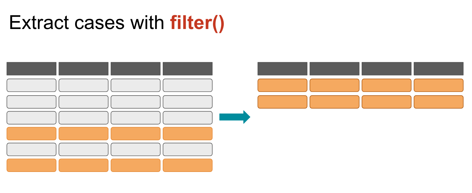
Filter works by extracting rows that meet a criteria you set.
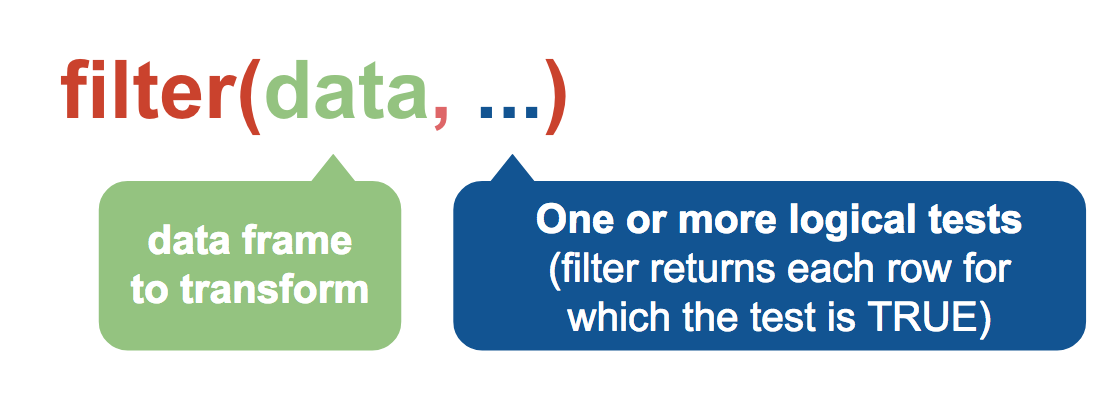
You pass the dataframe as a variable to filter() first and then you add any logical tests.
One = in R is the same as <- in that it assigns a value. Logical tests requires two, so == which tests for equal.
df1 <- filter(murders, Relationship_label=="Husband", VicAge > 60, Year==2016)

df2 <- filter(murders, Relationship_label=="Husband" & VicAge > 60 & Year==2016) # same as the line above

df3 <- filter(murders, Relationship_label %in% c("Husband", "Boyfriend") | Circumstance_label=="Lovers triangle")
Check out the new objects in the Environment window of RStudio.

Data frames df1 and df2 are exactly the same (Looking for cases in which Husbands were involved, the victim was older than 60, and occurred in 2016)– only 25 were found. Meanwhile d3 has nearly 32,000 cases in which a Husband or Boyfriend were involved or it was labeled by investigators as a lover’s triangle.
Logical Operators
| Operator | Description |
|---|---|
< |
Less than |
<= |
Less than or equal to |
> |
Greater than |
>= |
Greater than or equal to |
== |
Exactly equal to |
!= |
Not equal to |
!x |
Not x |
x | y |
x or y |
x & y |
x and y |
%in% |
Group membership |
isTRUE(x) |
Test if x is TRUE |
is.na(x) |
Test if x is NA |
!is.na(x) |
Test if x is not NA |
Test yourself
Can you use the logical operators and filter() to create df4 which has all the data for murders:
- in the District of Columbia
- That were solved in 2015 that involved Black victims
- in which Handgun - pistol, revolver, etc was victims between the ages of 18 and 21
Common mistakes
- Using
=instead of==
# WRONG
filter(murders, fstate_label="District of Columbia")

# RIGHT
filter(murders, fstate_label=="District of Columbia")- Forgetting quotes
# WRONG
filter(murders, fstate_label=District of Columbia)

# RIGHT
filter(murders, fstate_label="District of Columbia")- Collapsing multiple tests into one
# WRONG
filter(murders, 1980 < year < 1990)

# RIGHT
filter(murders, 1980 < year, year < 1990)- Stringing together many tests instead of using %in%
# Not WRONG but INEFFICIENT to type out
filter(murders, VicRace_label=="Black" | VicRace_label="Unknown" | VicRace_label=="Asian or Pacific Islander")

# RIGHT
filter(murders, VicRace_label %in% c("Black", "Unknown", "Asian or Pacific Islander"))
Alright, we’ve got new data frames narrowed down from 750,000 total to about 25 specific incidents of husbands murdering their partners who were older than 60 in 2016 and about 32,000 cases where either the husband or boyfriend was involved or the victim was involved in a love triangle.
We have 47 variables (aka columns) and we don’t need all of them for this basic analysis. Let’s narrow that down.
select()
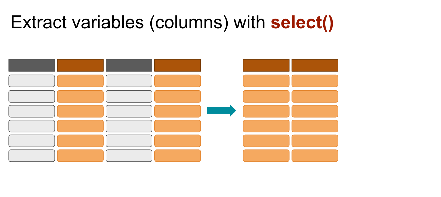
You simply list the column names after the data frame you want to extract from.
df1_narrow <- select(df1, State, Agency, Solved_label, Year)View(df1_narrow)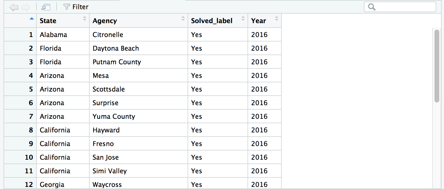
You can use a colon between column names if you want all the columns between.
df2_narrow <- select(df1, State, OffAge:OffRace_value, Weapon_label)View(df2_narrow)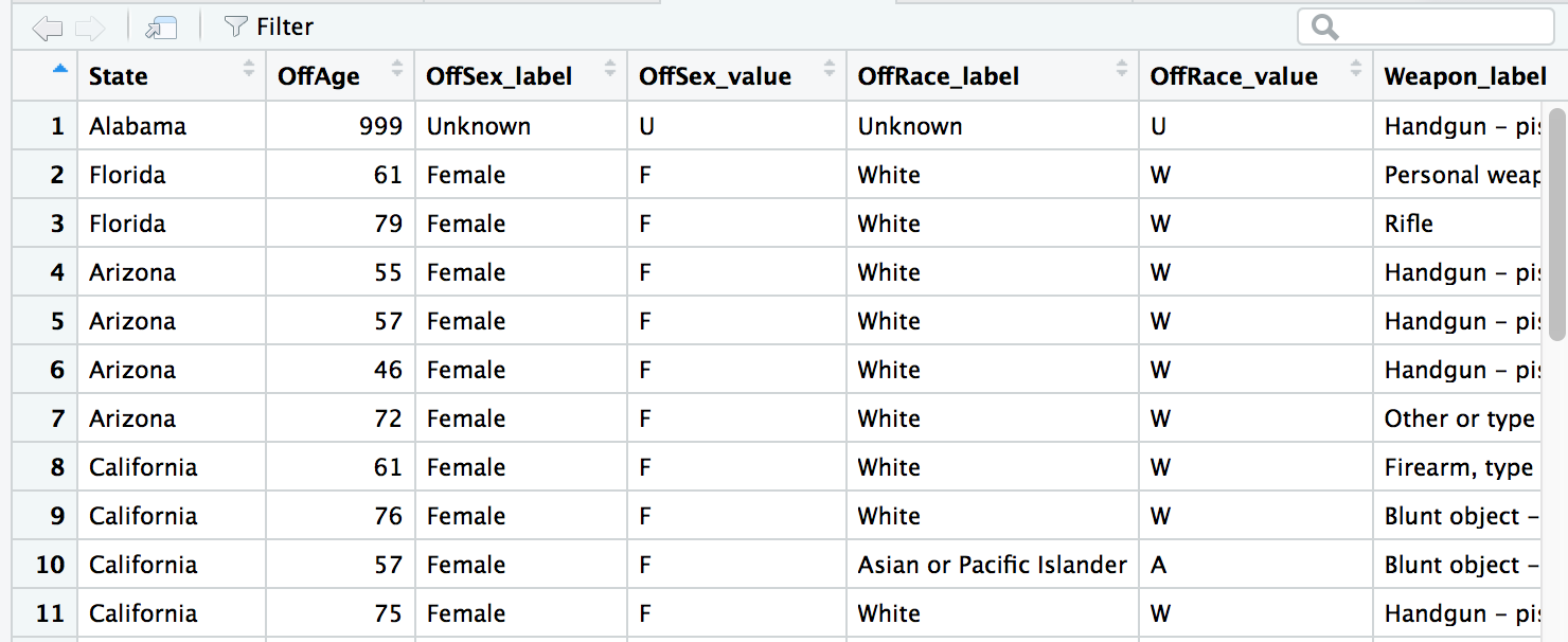
Use a - next to a column name to drop it (You can drop more than one column at a time, too).
# modifying the data frame created above
df3_narrow <- select(df2_narrow, -Weapon_label)
View(df3_narrow)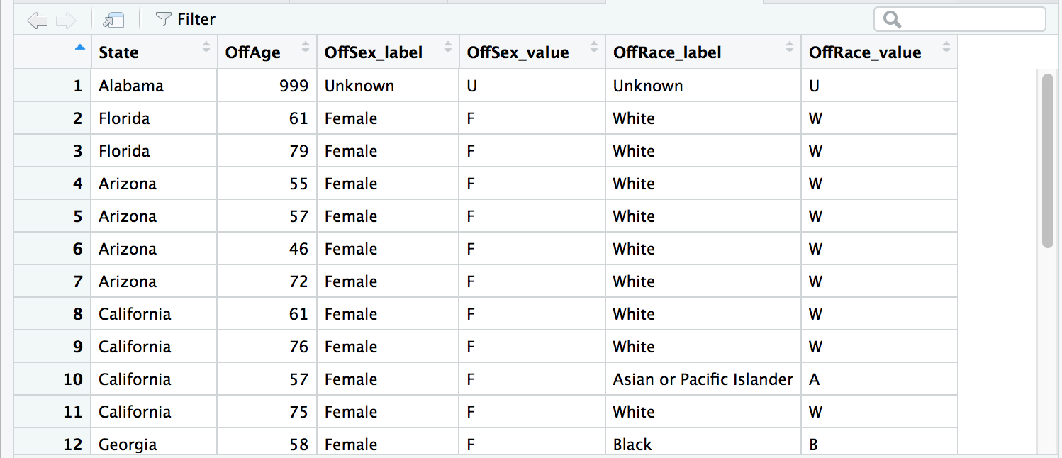
There are so many other functions you can use with select() to help make your life easier.
# This extracts all variables with names that contain "_label"

labels_only_columns <- select(murders, contains("_label"))
str(labels_only_columns)
Check out all the neat select() options here.
Great, let’s move on to the next verb.
arrange()
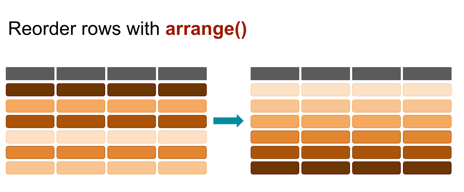
You can include more than one variable (column)– the first one will take priority but subsequent variables will serve as tie breakers.
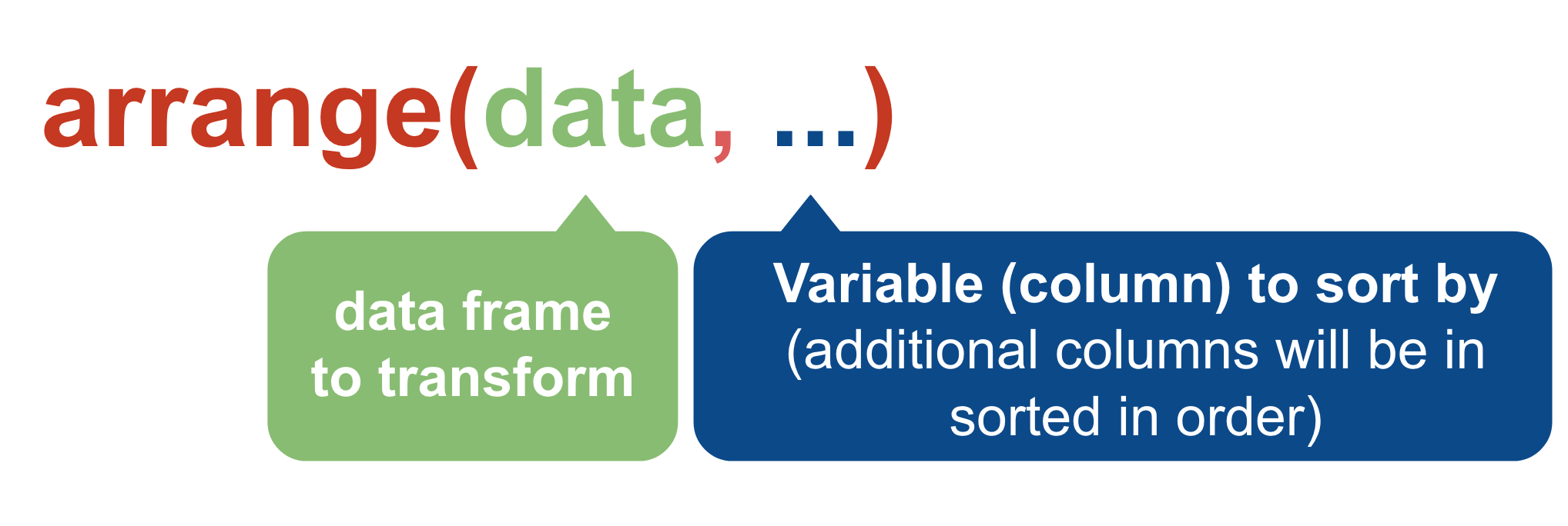
age_df1 <- arrange(murders, VicAge)

age_df2 <- arrange(murders, VicAge, OffAge)

age_df3 <- arrange(murders, VicAge, desc(OffAge))

# Same result as above
age_df3b <- arrange(murders, VicAge, -OffAge)
This will be very useful. Let’s move on to the next verb.
mutate()
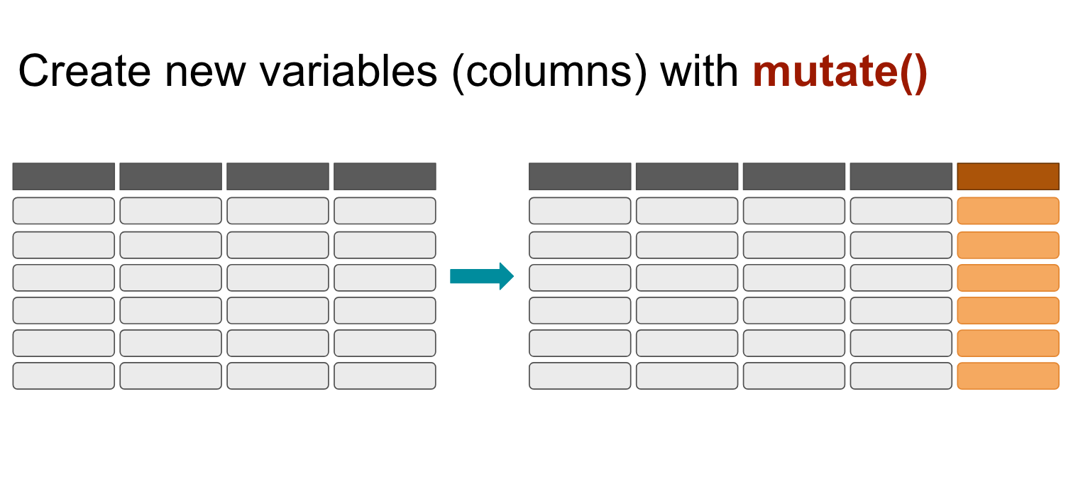
We can create new variables (new columns) with the mutate() function.
murders_ver2 <- mutate(murders,
                       age_difference=OffAge-VicAge)
View(murders_ver2)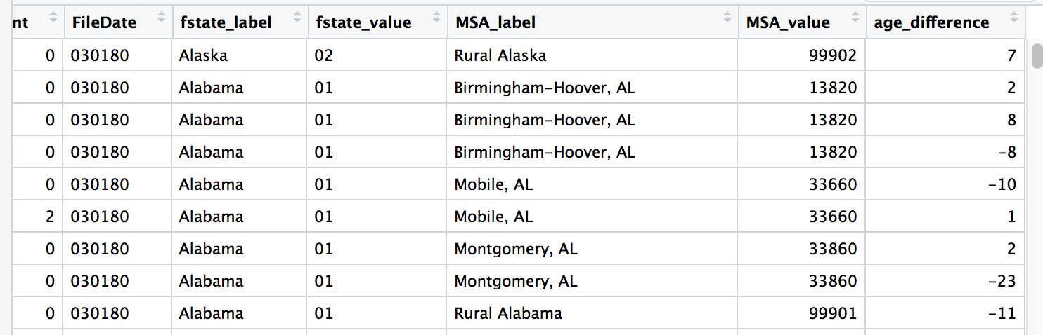
Arithmetic Operators
| Operator | Description |
|---|---|
+ |
Addition |
- |
Subtraction |
* |
Multiplication |
/ |
Division |
^ |
Exponentiation |
You can do more than just math in the context of mutate().
You can use case_when() in mutate() to create new values based on other values, kind of like an if_else statement.
# creates an age_difference column
# and creates a vic_category column that is populated with values depending on the VicRace_label column

murders_ver3 <- mutate(murders,
                       age_difference=OffAge-VicAge,
                       vic_category=case_when(
                         VicRace_label == "White" ~ "White",
                         VicRace_label != "White" ~ "Non-White"
                       ))
This is the first of a few times you’ll see the ~ (tilde) operator. It means it’s a one-sided formula, usually in statistical model formulas. It can be described as “depends on” You don’t need to really to understand why a tilde is necessary– only that this is how this particular function needs to be set up to work successfully.
There are two variables being created in the mutate() function separated by commas.
- one is age_difference which just subtracts the values in OffAge and VicAge.
- the other is vic_category that is either assigned “White” or “Non-White” depending on if the value of the column VicRace_label is “White” or not “White”.
View(murders_ver3)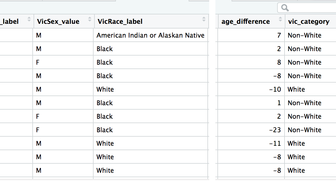
This is an example of a vectorized function in action. There are some really great ones like lag() and lead() and rank() and we might get into them later. In the meantime, here’s a neat list.
Rename
You can rename variables (columns) easily with the function rename()
colnames(df3_narrow)## [1] "State" "OffAge" "OffSex_label" "OffSex_value"
## [5] "OffRace_label" "OffRace_value"# OK, you see the column names above-- let's change a couple of them
df3_renamed <- rename(df3_narrow,
offender_gender=OffSex_label,
offender_age=OffAge)
colnames(df3_renamed)## [1] "State" "offender_age" "offender_gender" "OffSex_value"
## [5] "OffRace_label" "OffRace_value"You can also rename variables (columns) with the select() function. This is just a way to cut down on extra lines of code
colnames(df3_narrow)## [1] "State" "OffAge" "OffSex_label" "OffSex_value"
## [5] "OffRace_label" "OffRace_value"# Keeping only the State and offender gender and age columns but renaming the OffSex_label and OffAge columns
df4_renamed <- select(df3_narrow,
State,
offender_gender=OffSex_label,
offender_age=OffAge)
df4_renamed## State offender_gender offender_age
## 1 Alabama Unknown 999
## 2 Florida Female 61
## 3 Florida Female 79
## 4 Arizona Female 55
## 5 Arizona Female 57
## 6 Arizona Female 46
## 7 Arizona Female 72
## 8 California Female 61
## 9 California Female 76
## 10 California Female 57
## 11 California Female 75
## 12 Georgia Female 58
## 13 Kentucky Female 77
## 14 Kentucky Female 67
## 15 Michigan Female 72
## 16 Michigan Female 72
## 17 Mississippi Female 46
## 18 New Mexico Male 83
## 19 Oklahoma Female 58
## 20 Pennsylvania Female 57
## 21 Rhodes Island Female 57
## 22 South Carolina Female 72
## 23 South Carolina Female 76
## 24 Tennessee Female 63
## 25 Texas Female 71summarize()
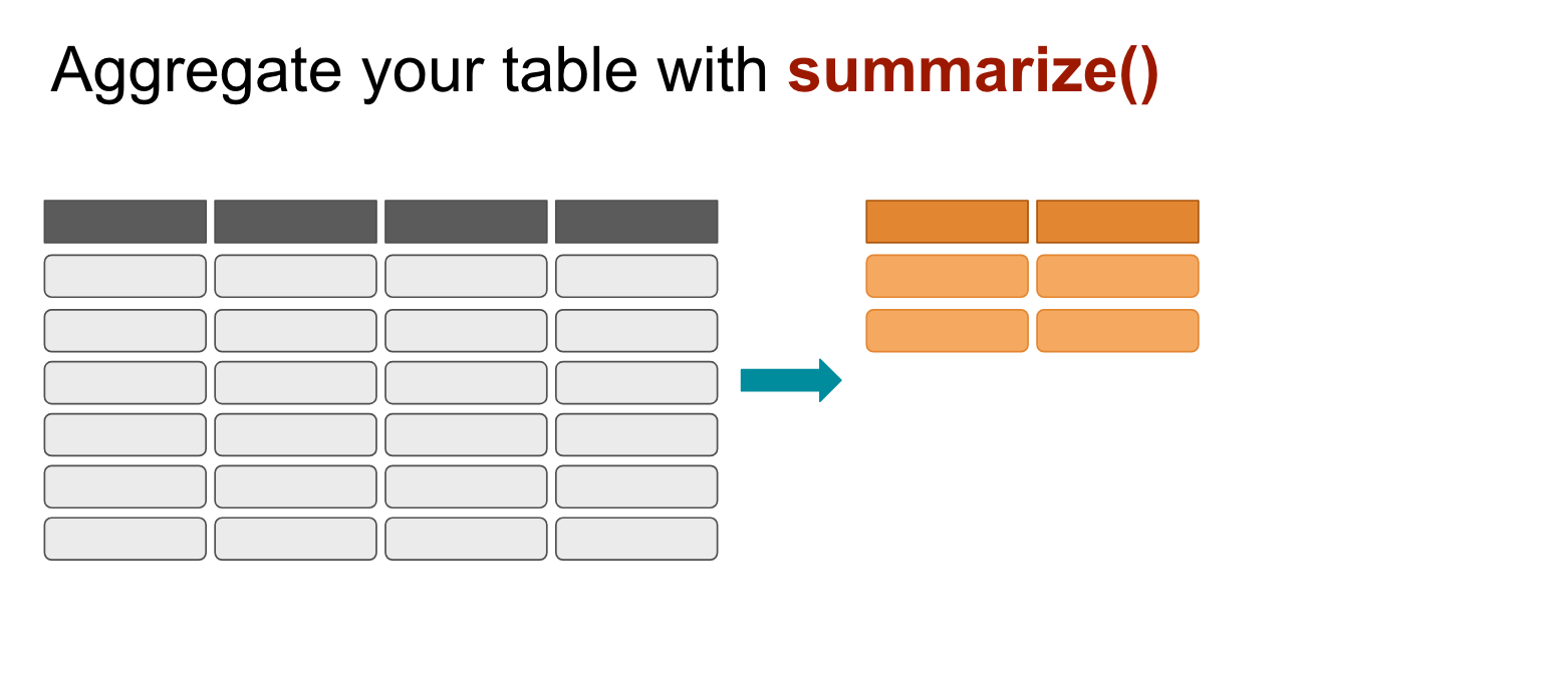
This is the equivalent of creating a pivot table in Excel.
You’re aggregating the whole table into something simplified.
summarize(murders, average_victim_age=mean(VicAge))## average_victim_age
## 1 47.96203You can create a table of summaries.
summarize(murders,
          average_victim_age=mean(VicAge),
          average_offender_age=mean(OffAge))
## average_victim_age average_offender_age
## 1 47.96203 352.7295There’s something wrong with the average_offender_age value. Can you figure out what happened?
Summarize the data frame murders
summarize(murders,
          first=min(Year),
          last=max(Year),
          metro_areas=n_distinct(MSA_label),
          cases=n())
## first last metro_areas cases
## 1 1976 2016 409 752313group_by()
You can aggregate data by groups before summarizing.
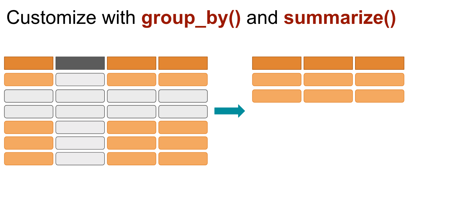
# This is the same process as before but we're telling R to group up the metro areas before summarizing the data

murders <- group_by(murders, MSA_label)

summarize(murders,
          first=min(Year),
          last=max(Year),
          cases=n())
## # A tibble: 409 x 4
## MSA_label first last cases
## <fct> <dbl> <dbl> <int>
## 1 Abilene, TX 1976 2016 366
## 2 Akron, OH 1976 2016 1080
## 3 Albany, GA 1976 2016 633
## 4 Albany-Schenectady-Troy, NY 1976 2016 829
## 5 Albuquerque, NM 1976 2016 2374
## 6 Alexandria, LA 1976 2016 576
## 7 Allentown-Bethlehem-Easton, PA-NJ 1976 2016 882
## 8 Altoona, PA 1976 2016 120
## 9 Amarillo, TX 1976 2016 724
## 10 Ames, IA 1978 2016 26
## # ... with 399 more rowsThis might be a tough concept to fully understand at first, but we’ll go over a few more examples soon so it will hopefully make more sense.
Also, I want to point out that the opposite of group_by() is ungroup() which you might need later on as you progress.
But let’s get over some very useful functionality that comes with the dplyr package.
pipe %>%
Data analyses will most often involve more than one step.
We’re going to over some options on how to approach multi-step processes with this data set and then we’ll go over the best way to deal with them.
Description of theoretical process to run on the murders data frame:
- Extract rows for cases that happened in Washington DC, then
- Group case by year and then
- Count the number of cases
- Arrange the by decreasing cases
Option 1
Build out a new dataframe for each step.
dc_annual_murders1 <- filter(murders, State=="District of Columbia")
dc_annual_murders2 <- group_by(dc_annual_murders1, Year)
dc_annual_murders3 <- summarize(dc_annual_murders2, total=n())
dc_annual_murders4 <- arrange(dc_annual_murders3, desc(total))

# looking at the first 6 rows of data

head(dc_annual_murders4)
## # A tibble: 6 x 2
## Year total
## <dbl> <int>
## 1 1991 489
## 2 1990 481
## 3 1992 450
## 4 1989 439
## 5 1993 423
## 6 1994 417Option 2
Do it all in one line by nesting functions.
dc_annual_murders <- arrange(summarize(group_by(filter(murders, State=="District of Columbia"), Year), total=n()), desc(total))

# looking at the first 6 rows of data

head(dc_annual_murders)
## # A tibble: 6 x 2
## Year total
## <dbl> <int>
## 1 1991 489
## 2 1990 481
## 3 1992 450
## 4 1989 439
## 5 1993 423
## 6 1994 417These options aren’t great because the first one involves just way too much typing, even if it’s pretty clear to an outside reader what’s happening to the data frame. The second one is no good because, while it’s efficient with coding, it’s way too difficult to follow what’s happening to the data.
Let’s talk about the pipe operator %>%
You might have noticed that all the functions from dplyr all structured similarly: The first argument is always the data frame.
It takes in a data frame and spits out a data frame.
This function structure is what allows for something like the %>% to work.

These commands do the same thing. Give it a try.
filter(murders, OffAge==2)## # A tibble: 3 x 47
## # Groups: MSA_label [3]
## ID CNTYFIPS Ori State Agency AGENCY_A Agentype_label Agentype_value
## <fct> <fct> <fct> <fct> <fct> <fct> <fct> <dbl>
## 1 1977… "13121 … GA06… Geor… "East… " … Municipal pol… 3
## 2 1979… "36061 … NY03… New … "New … " … Municipal pol… 3
## 3 2015… "18089 … IN04… Indi… "Gary… " … Municipal pol… 3
## # ... with 39 more variables: Source_label <fct>, Source_value <dbl>,
## # Solved_label <fct>, Solved_value <dbl>, Year <dbl>, Month_label <fct>,
## # Month_value <dbl>, Incident <dbl>, ActionType <fct>,
## # Homicide_label <fct>, Homicide_value <fct>, Situation_label <fct>,
## # Situation_value <fct>, VicAge <dbl>, VicSex_label <fct>,
## # VicSex_value <fct>, VicRace_label <fct>, VicRace_value <fct>,
## # VicEthnic <fct>, OffAge <dbl>, OffSex_label <fct>, OffSex_value <fct>,
## # OffRace_label <fct>, OffRace_value <fct>, OffEthnic <fct>,
## # Weapon_label <fct>, Weapon_value <dbl>, Relationship_label <fct>,
## # Relationship_value <fct>, Circumstance_label <fct>,
## # Circumstance_value <dbl>, Subcircum <fct>, VicCount <dbl>,
## # OffCount <dbl>, FileDate <fct>, fstate_label <fct>,
## # fstate_value <fct>, MSA_label <fct>, MSA_value <dbl>murders %>% filter(OffAge==2)## # A tibble: 3 x 47
## # Groups: MSA_label [3]
## ID CNTYFIPS Ori State Agency AGENCY_A Agentype_label Agentype_value
## <fct> <fct> <fct> <fct> <fct> <fct> <fct> <dbl>
## 1 1977… "13121 … GA06… Geor… "East… " … Municipal pol… 3
## 2 1979… "36061 … NY03… New … "New … " … Municipal pol… 3
## 3 2015… "18089 … IN04… Indi… "Gary… " … Municipal pol… 3
## # ... with 39 more variables: Source_label <fct>, Source_value <dbl>,
## # Solved_label <fct>, Solved_value <dbl>, Year <dbl>, Month_label <fct>,
## # Month_value <dbl>, Incident <dbl>, ActionType <fct>,
## # Homicide_label <fct>, Homicide_value <fct>, Situation_label <fct>,
## # Situation_value <fct>, VicAge <dbl>, VicSex_label <fct>,
## # VicSex_value <fct>, VicRace_label <fct>, VicRace_value <fct>,
## # VicEthnic <fct>, OffAge <dbl>, OffSex_label <fct>, OffSex_value <fct>,
## # OffRace_label <fct>, OffRace_value <fct>, OffEthnic <fct>,
## # Weapon_label <fct>, Weapon_value <dbl>, Relationship_label <fct>,
## # Relationship_value <fct>, Circumstance_label <fct>,
## # Circumstance_value <dbl>, Subcircum <fct>, VicCount <dbl>,
## # OffCount <dbl>, FileDate <fct>, fstate_label <fct>,
## # fstate_value <fct>, MSA_label <fct>, MSA_value <dbl>In essence, a %>% is the grammatical equivalent of and then….
Again, a description of the theoretical process:
- Extract rows for cases that happened in Washington DC, then
- Group case by year and then
- Count the number of cases
- Arrange the by decreasing cases
Option 3
Use the %>% pipe
filter(murders, State=="District of Columbia") %>%
  group_by(Year) %>%
  summarize(total=n()) %>%
  arrange(desc(total)) %>%
  head()
## # A tibble: 6 x 2
## Year total
## <dbl> <int>
## 1 1991 489
## 2 1990 481
## 3 1992 450
## 4 1989 439
## 5 1993 423
## 6 1994 417So readable and simple, right?
Here’s the shortcut to type %>% in RStudio:
- Mac: Cmd + Shift + M
- Windows: Ctrl + Shift + M
Why “M”? I think it’s because the pipe was first introduced in the magrittr package by Stefan Milton Bache.
Mutate again
There are a lot of interesting things you can do with mutate().
Let’s try out lag() within mutate() – it lets you do math based on the previous row of a vector.
For example, in the data frame above we’ve got the number of murders in DC. With lag() and some math, we can calculate the difference in the number of murders year over year.
# We can keep the code from before but now we add a new mutate line
filter(murders, State=="District of Columbia") %>%
  group_by(Year) %>%
  summarize(total=n()) %>%
  mutate(previous_year=lag(total)) %>%
  mutate(change=total-previous_year)
## # A tibble: 35 x 4
## Year total previous_year change
## <dbl> <int> <int> <int>
## 1 1976 203 NA NA
## 2 1977 202 203 -1
## 3 1978 196 202 -6
## 4 1979 171 196 -25
## 5 1980 180 171 9
## 6 1981 232 180 52
## 7 1982 204 232 -28
## 8 1983 188 204 -16
## 9 1984 175 188 -13
## 10 1985 149 175 -26
## # ... with 25 more rowsSo mutate() returns a vector the same length as the input.
We summarized the code and then we mutated a new column based on lag() and then we mutated a second column based on the new column and the old column.
You can use mutate more than once
# Here's an example of the same code above but with mutate called just once
# previous_year was able to be referenced a second time because it was created in first
years <- filter(murders, State=="District of Columbia") %>%
  group_by(Year) %>%
  summarize(total=n()) %>%
  mutate(previous_year=lag(total), change=previous_year-total)

years
## # A tibble: 35 x 4
## Year total previous_year change
## <dbl> <int> <int> <int>
## 1 1976 203 NA NA
## 2 1977 202 203 1
## 3 1978 196 202 6
## 4 1979 171 196 25
## 5 1980 180 171 -9
## 6 1981 232 180 -52
## 7 1982 204 232 28
## 8 1983 188 204 16
## 9 1984 175 188 13
## 10 1985 149 175 26
## # ... with 25 more rowsSo mutate() works when the formula you pass it returns a vectorized output. For example, if a vector has 10 instances in it, then the formula needs to output 10 instances, too.
Passing it a formula like sum() would confuse it.
years %>% mutate(all_murders=sum(total))## # A tibble: 35 x 5
## Year total previous_year change all_murders
## <dbl> <int> <int> <int> <int>
## 1 1976 203 NA NA 8209
## 2 1977 202 203 1 8209
## 3 1978 196 202 6 8209
## 4 1979 171 196 25 8209
## 5 1980 180 171 -9 8209
## 6 1981 232 180 -52 8209
## 7 1982 204 232 28 8209
## 8 1983 188 204 16 8209
## 9 1984 175 188 13 8209
## 10 1985 149 175 26 8209
## # ... with 25 more rowsThis is what differentiates mutate() from summarize().
Summary functions
What summarize() does is it takes a vector as an input, and returns a single value as output. Like sum() did in the previous example.
Here are some examples of summary functions:
| Function | Description |
|---|---|
mean(x) |
Mean (average). mean(c(1,10,100,1000)) returns 277.75 |
median(x) |
Median. median(c(1,10,100,1000)) returns 55 |
sd(x) |
Standard deviation. sd(c(1,10,100,1000)) returns 483.57 |
quantile(x, probs) |
Where x is the numeric vector whose quantiles are desired and probs is a numeric vector with probabilities |
range(x) |
Range. range(c(1,10,100,1000)) returns c(1, 1000) and diff(range(c(1,10,100,1000))) returns 999 |
sum(x) |
Sum. sum(c(1,10,100,1000)) returns 1111 |
min(x) |
Minimum. min(c(1,10,100,1000)) returns 1 |
max(x) |
Maximum. max(c(1,10,100,1000)) returns 1000 |
abs(x) |
Absolute value. abs(-8) returns 8 |
Here are some examples of summary functions specific to dplyr and summarize() – Learn about the others.
| Function | Description |
|---|---|
n() |
returns the number of values/rows |
n_distinct() |
returns number of uniques |
first() |
Only returns the first value within an arranged group |
last() |
Only returns the last value within an arranged group |
nth() |
Only returns the nth location of a vector |
group_by() again
Let’s put together everything we’ve learned by calculating percentages.
You can use group_by() on more than one variable (column).
Let’s go over the difference, really quick.
We can summarize the data by how many men were murdered versus women by
murders %>%
  group_by(VicSex_label) %>%
  summarize(total=n())
## # A tibble: 3 x 2
## VicSex_label total
## <fct> <int>
## 1 Female 169028
## 2 Male 582092
## 3 Unknown 1193By grouping VicSex_label we got the counts (n()) for all the instances available in that variable.
We can add another variable (column) name into the group_by() to drill deeper. Watch what happens when we add State.
murders %>%
  group_by(State, VicSex_label) %>%
  summarize(total=n())
## # A tibble: 147 x 3
## # Groups: State [?]
## State VicSex_label total
## <fct> <fct> <int>
## 1 Alaska Female 565
## 2 Alaska Male 1385
## 3 Alaska Unknown 2
## 4 Alabama Female 3586
## 5 Alabama Male 11955
## 6 Alabama Unknown 146
## 7 Arkansas Female 2019
## 8 Arkansas Male 6049
## 9 Arkansas Unknown 28
## 10 Arizona Female 3252
## # ... with 137 more rowsInteresting, right? The structure for the data here might be foreign to you. As it stands, this data is considered tidy. Each variable is a column and each observation (or case) is a row. This makes it easier to analyze the data in R and create charts.
But you’re probably used to data that looks like
## # A tibble: 51 x 4
## # Groups:   State [51]
##    State                Female  Male Unknown
##    <fct>                 <int> <int>   <int>
##  1 Alaska                  565  1385       2
##  2 Alabama                3586 11955     146
##  3 Arkansas               2019  6049      28
##  4 Arizona                3252 11203      29
##  5 California            21826 92756      38
##  6 Colorado               2233  5476       5
##  7 Connecticut            1394  4139       5
##  8 District of Columbia   1041  7155      13
##  9 Delaware                399  1048      NA
## 10 Florida               10699 32632     128
## # ... with 41 more rows
And that’s fine, too, for presentation. We’ll get into how to do this later in the next chapter or so.
The prior tidy structure makes it easier to run calculations such as percentages, however.
Percents
Now we get a chance to chain together all the verbs we’ve used
percent_murders <- murders %>%
  group_by(State, VicSex_label) %>%
  summarize(total=n()) %>%
  # okay, we've got the total, now we can do some math with mutate
  mutate(percent=total/sum(total, na.rm=T)*100)
  # did you notice the na.rm=T added to the sum function? This removes NAs
  # That's necessary because if you have a single NA then it will not sum correctly (thanks, statisticians!)

percent_murders
## # A tibble: 147 x 4
## # Groups: State [51]
## State VicSex_label total percent
## <fct> <fct> <int> <dbl>
## 1 Alaska Female 565 28.9
## 2 Alaska Male 1385 71.0
## 3 Alaska Unknown 2 0.102
## 4 Alabama Female 3586 22.9
## 5 Alabama Male 11955 76.2
## 6 Alabama Unknown 146 0.931
## 7 Arkansas Female 2019 24.9
## 8 Arkansas Male 6049 74.7
## 9 Arkansas Unknown 28 0.346
## 10 Arizona Female 3252 22.5
## # ... with 137 more rowsInteresting. We can use more dplyr() verbs to find something of interest. Like, which states have a higher percent of women murdered?
percent_murders_women <- murders %>%
  group_by(State, VicSex_label) %>%
  summarize(total=n()) %>%
  mutate(percent=total/sum(total, na.rm=T)*100) %>%
  filter(VicSex_label=="Female") %>%
  arrange(-percent)

# Using the DT (DataTables) library that lets us create searchable tables with the plug-in for jQuery
# If you don't have DT installed yet, uncomment the line below and run it
#install.packages("DT")

library(DT)
datatable(percent_murders_women)
Congratulations, we’ve gone through a bunch of ways to analyze data.
Now that we’ve got the tools, let’s interrogate the data further using a couple other methods involving tidying and joining data.
Your turn
Challenge yourself with these exercises so you’ll retain the knowledge of this section.
Instructions on how to run the exercise app are on the intro page to this section.
© Copyright 2018, Andrew Ba Tran