Geolocating data
Geolocating addresses in R
We’re going to start with geolocating municipal police stations in Connecticut.
We’ll be using the ggmap package for a lot of functions, starting with geolocating addresses with Google Maps.
# if you don't have the following packages installed, uncomment and run the lines below

#install.packages(c("dplyr", "ggplot2", "tidyr", "ggmap", "DT", "knitr", "readr"))

library(readr)
library(dplyr)
library(ggplot2)
library(tidyr)
library(ggmap)
library(DT)
library(knitr)
After we import the data, let’s use the glimpse() function which lists out the variables for the data frame.
stations <- read_csv("data/Police_Departments.csv")## Parsed with column specification:
## cols(
## NAME = col_character(),
## DESCRIPTION = col_character(),
## TELEPHONE = col_character(),
## ADDRESS = col_character(),
## ADDRESS2 = col_character(),
## CITY = col_character(),
## STATE = col_character(),
## ZIP = col_integer(),
## ZIPP4 = col_integer()
## )glimpse(stations)## Observations: 185
## Variables: 9
## $ NAME <chr> "AMTRAK POLICE DEPARTMENT", "ANDOVER POLICE DEPART...
## $ DESCRIPTION <chr> "OTHER", "MUNICIPAL", "COLLEGE OR UNIVERSITY", "CO...
## $ TELEPHONE <chr> "203-773-6000", "860-742-0235", "860-405-9088", "8...
## $ ADDRESS <chr> "50 UNION AVENUE", "17 SCHOOL ROAD", "1084 SHENNEC...
## $ ADDRESS2 <chr> NA, NA, NA, NA, NA, NA, NA, NA, NA, NA, NA, NA, NA...
## $ CITY <chr> "NEW HAVEN", "ANDOVER", "GROTON", "HARTFORD", "NEW...
## $ STATE <chr> "CT", "CT", "CT", "CT", "CT", "CT", "CT", "CT", "C...
## $ ZIP <int> 6519, 6232, 6340, 6103, 6050, 6410, 6413, 6415, 61...
## $ ZIPP4 <int> 1754, 1526, 6048, 1207, 2439, 2249, 2115, 1230, 16...To find the latitude and longitude of an address, we need a full address like you would put into Google Maps. This data frame has a separate column for each piece of the address.
We need a single column for addresses, so we’ll concatenate ADDRESS, CITY, STATE, and ZIP.
Did you notice the zip code is numeric and has only 4 digits out of 5 for zip code? That’s because Connecticut zip codes all start with 0. We’ll need to put that 0 back for the geocoding to work successfully.
stations <- stations %>%
  mutate(ZIP=paste0("0", as.character(ZIP))) %>%
  mutate(location = paste0(ADDRESS, ", ", CITY, ", CT ", ZIP))
The function to geocode a single address is geocode() but we’ve got a bunch of addresses, so we can use mutate_geocode().
geo <- mutate_geocode(stations, location)# If it's taking too long, you can cancel and load the output by uncommenting the line below
geo <- read_csv("data/geo_stations.csv")
# Bringing over the longitude and latitude data
stations$lon <- geo$lon
stations$lat <- geo$latThis is using Google’s service, and last I checked there were about 2,500 queries allowed per day if you don’t have a key. If you do get a key, check out the documentation at the bottom of this page.
Also did you know that Google let’s you reverse geocode?
If you pass latitude and longitude data to revgeocode() it will return an address.
revgeocode(c(lon = -77.030137, lat = 38.902986))## address
## 1 NAPlotting points with ggplot2
Let’s pull town shapes for Connecticut with tigris.
# If you don't have tigris or ggplot2 or sf installed yet, uncomment and run the line below
#install.packages("tigris", "sf", "ggplot2")

library(tigris)
library(sf)
library(ggplot2)

# set sf option

options(tigris_class = "sf")

ct <- county_subdivisions("CT", cb=T)

#If cb is set to TRUE, download a generalized (1:500k) counties file. Defaults to FALSE (the most detailed TIGER file).

ggplot(ct) +
  geom_sf() +
  theme_void() +
  theme(panel.grid.major = element_line(colour = 'transparent')) +
  labs(title="Connecticut towns")
Okay, we’ve got the shape file.
We just add the geolocated points like it was dots on a chart. Because that’s essentially what latitude and longitude is.
ggplot(ct) +
  geom_sf() +
  geom_point(data=stations, aes(x=lon, y=lat), color="blue") +
  theme_void() +
  theme(panel.grid.major = element_line(colour = 'transparent')) +
  labs(title="Police stations")
Alright, I’ll throw in grouping for Description.
And generate some random numbers for staffing for each station so we can make some circle plots.
set.seed(7)

stations$staff <- sample(200, size=nrow(stations), replace=T)

ggplot(ct) +
  geom_sf(fill="transparent") +
  geom_point(data=stations, aes(x=lon, y=lat, size=staff, color=DESCRIPTION),  fill="white", shape=1) +
  theme_void() +
  theme(panel.grid.major = element_line(colour = 'transparent')) +
  labs(title="Police stations in Connecticut") +
  coord_sf()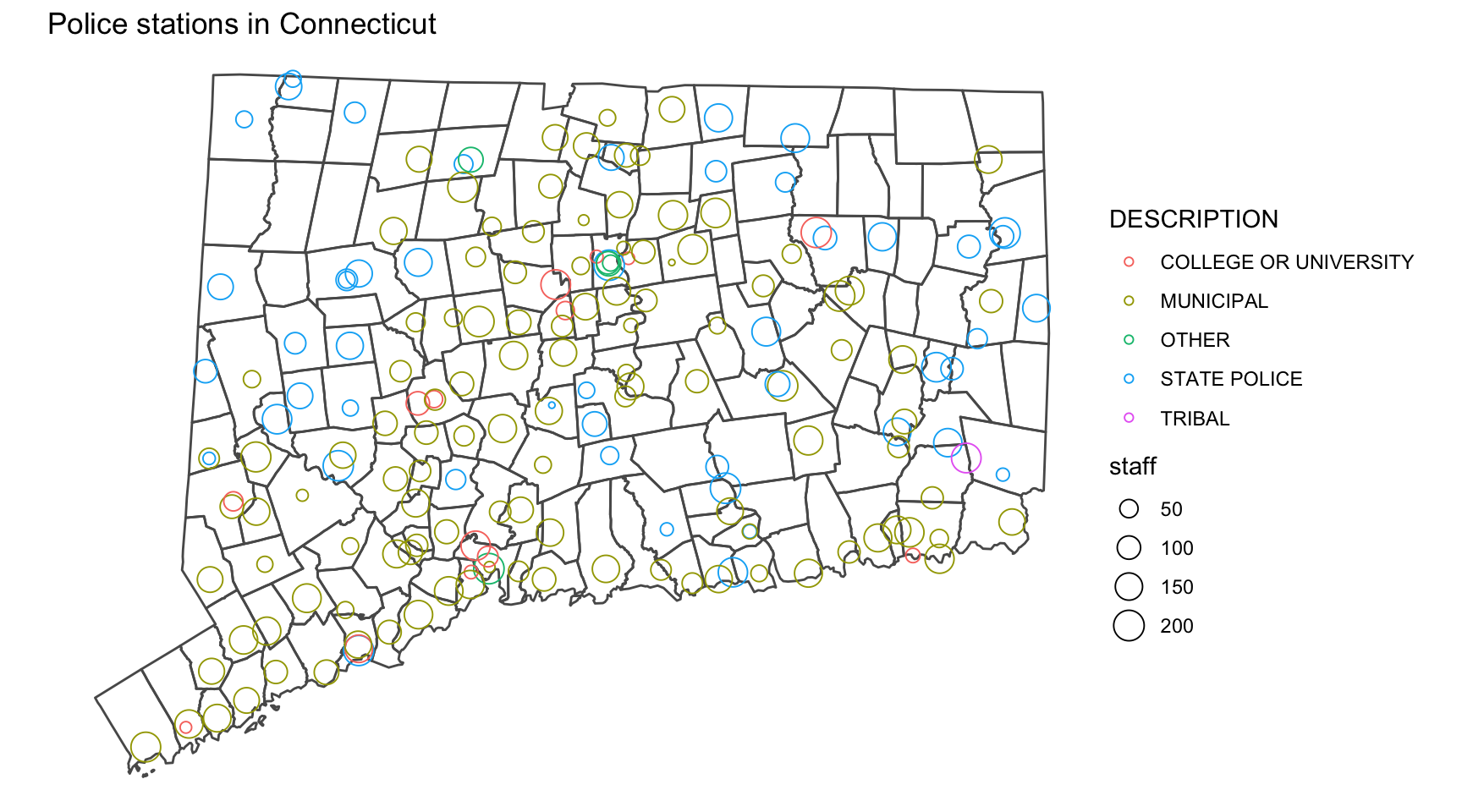
I also threw in coord_sf() in there at the end. It makes sures that all layer are using a common CRS. It sets it based on the first layer.
You can set other projections easily.
© Copyright 2018, Andrew Ba Tran