R for Journalists > Importing/Exporting data > CSV files

CSV files

Comma separated files are the most common way to save spreadsheets that doesn’t require a paid program from Microsoft to open.

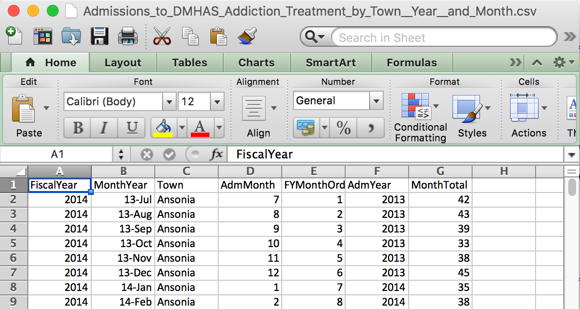
What a csv file looks like

CSV file names end with a .csv

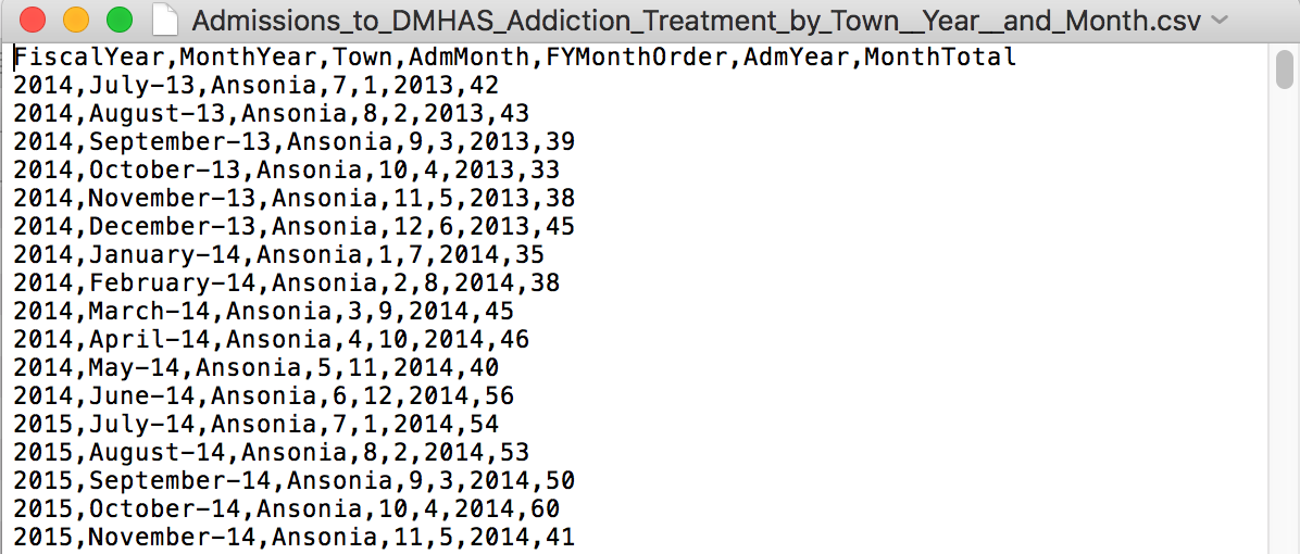
What a csv file looks like on the inside

This explains the values separated with commas part of the file name.

Importing CSV files

Importing CSV is part of base R, no package needed
But we’re going to use a package anyway, readr

Two ways to get data

If you have the URL address
- If the csv file exists on the internet, you don’t have to download it to your local machine and then import it, you can import it to R directly from the web using the link
If you have the file on your computer

Get the URL

If you have the link to a CSV file, right click the link of the data and click Copy Link Address. This data set can be found on the Connecticut Open Data Portal.

read.csv()

The Base R function to import a CSV file is read.csv(). Just put the URL address in quotation marks and add the stringsAsFactors=F (In this code we’re using the function head()– this returns 6 rows by default, but we want to look at 10, so we’ll specify that when we call the function head(data, 10))

df_csv <- read.csv("https://data.ct.gov/api/views/iyru-82zq/rows.csv?accessType=DOWNLOAD", stringsAsFactors=F)
head(df_csv, 10)

##    FiscalYear    MonthYear    Town AdmMonth FYMonthOrder AdmYear
## 1        2014      July-13 Ansonia        7            1    2013
## 2        2014    August-13 Ansonia        8            2    2013
## 3        2014 September-13 Ansonia        9            3    2013
## 4        2014   October-13 Ansonia       10            4    2013
## 5        2014  November-13 Ansonia       11            5    2013
## 6        2014  December-13 Ansonia       12            6    2013
## 7        2014   January-14 Ansonia        1            7    2014
## 8        2014  February-14 Ansonia        2            8    2014
## 9        2014     March-14 Ansonia        3            9    2014
## 10       2014     April-14 Ansonia        4           10    2014
##    MonthTotal
## 1          42
## 2          43
## 3          39
## 4          33
## 5          38
## 6          45
## 7          35
## 8          38
## 9          45
## 10         46

The other way to import the data: Download it

When you right click on the link, instead of clicking Copy Link Address– this time, click Save Link As…

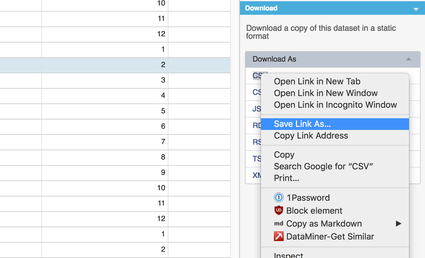
Save to your working directory.

After saving to the directory, click on the circle arrow on the right to refresh the files to make sure it’s there.

Recall: How to change directories in RStudio

Either by typing setwd("/directory/where/you/want") or by clicking in the menu up top Session > Set Working Directory > Choose Directory…

Importing local csv data

Just like before, except instead of the URL, it’s the name of the file.

Note: This will only work if the working directory is set to where the csv file is.

df_csv <- read.csv("data/Admissions_to_DMHAS_Addiction_Treatment_by_Town__Year__and_Month.csv", stringsAsFactors=F)

stringsAsFactors=F

Why?

Blame statisticians.

Back when R was created the users weren’t using it as we use it now, with all these different strings.

What happens when you don’t use stringsAsFactors=F

df_csv <- read.csv("data/Admissions_to_DMHAS_Addiction_Treatment_by_Town__Year__and_Month.csv")
str(df_csv)

## 'data.frame':    3420 obs. of  7 variables:
##  $ FiscalYear  : int  2014 2014 2014 2014 2014 2014 2014 2014 2014 2014 ...
##  $ MonthYear   : Factor w/ 36 levels "April-14","April-15",..: 16 4 34 31 28 7 13 10 22 1 ...
##  $ Town        : Factor w/ 102 levels "Ansonia","Berlin",..: 1 1 1 1 1 1 1 1 1 1 ...
##  $ AdmMonth    : int  7 8 9 10 11 12 1 2 3 4 ...
##  $ FYMonthOrder: int  1 2 3 4 5 6 7 8 9 10 ...
##  $ AdmYear     : int  2013 2013 2013 2013 2013 2013 2014 2014 2014 2014 ...
##  $ MonthTotal  : int  42 43 39 33 38 45 35 38 45 46 ...

Using read_csv() from the readr package

readr is a package that read rectangular data quickly and assumes characters are strings and not factors by default.

## If you don't have readr installed yet, uncomment and run the line below
#install.packages("readr")
library(readr)
df_csv <- read_csv("data/Admissions_to_DMHAS_Addiction_Treatment_by_Town__Year__and_Month.csv")

## Parsed with column specification:
## cols(
##   FiscalYear = col_double(),
##   MonthYear = col_character(),
##   Town = col_character(),
##   AdmMonth = col_double(),
##   FYMonthOrder = col_double(),
##   AdmYear = col_double(),
##   MonthTotal = col_double()
## )

As you can see, the read_csv() function interpreted the MonthYear and Town columns as characters and not as Factors as read.csv() did.

Exporting CSV files

When you’re done analyzing or transforming your data, you can save your dataframe as a CSV file with write_csv() from the readr package.

# Pass the write_csv() function the name of the dataframe and what you want to call the file
write_csv(df_csv, "transformed_data.csv")

The file will save to your working directory, but you can specify sub directories with the function.

# Pass the write_csv() function the name of the dataframe and what you want to call the file
write_csv(df_csv, "data/transformed_data.csv")

Exporting data frames with `NA`

Weird quirk alert: Exported files will include NAs so to replace them, pass the variable na="whatever".

# This replaces the NAs with blanks
write_csv(df_csv, "data/transformed_data.csv", na="")

Your turn

Challenge yourself with these exercises so you’ll retain the knowledge of this section.

Instructions on how to run the exercise app are on the intro page to this section.