Murders case study
The FBI has tracked more than 750,000 murders in 40 years across the country. And that’s not counting the police departments that refuse to send them their homicide statistics.
Thomas Hargrove was a national correspondent for the Scripps Howard News Service, where he developed an algorithm that uses FBI homicide data to identify areas of murders that had an elevated probability of containing serial killings. His work helped convince officials in Ohio and Indiana to begin investigating specific strangulation cases in 2010. The case lead to the arrest of Darren Deon Vann, who confessed to killing women for decades and took police to abandoned properties in Gary, Indiana to recover undiscovered victims.
Hargrove has since retired and runs the Murder Accountability Project.
We’re going to go over his algorithm and try to reproduce it.
This is just an algorithm based on the available variables in the data. The results cannot match good, natural police work. The methodology discussed in this section may produce false results either by making false matches between unrelated cases or by failing to detect known linked cases. Further investigation should be mandatory if reporting on findings to avoid unnecessary overreaction. The ultimate authority on whether homicide cases should be linked rests with the local law enforcement agencies which investigate crimes and with the appropriate courts of criminal law.
Let’s start by looking at the case of “Green River Killer” Gary Ridgway.
Ridgway’s slayings began in 1982, when young runaways and prostitutes began disappearing from state Route 99 in south King County, Washington. He brought many of them to his home and strangled them, then left them in woodsy, remote sites. The first few bodies turned up along the now-notorious Green River.
Ridgway told investigators he killed as many as 75-80 women along Route 99 in south King County, Washington. He was convicted and received multiple life sentences.
How would we find his victims in our data set?
There were definitely patterns.
- King County, Washington
- Time span was between 1982 and 2001
- Female victims
- Victims often strangled
- Found in remote locations
Import the data in first.
library(dplyr)
library(tidyr)
library(DT)
source("import_murders.R")
Let’s apply the criteria above to the data set.
There’s a problem at the moment.
There’s no county variable. There’s a county FIPS code column, but not one identifying the name of the county.
I’ve uploaded a relationship file for you.
# If you don't have readr installed yet, uncomment and run the line below
#install.packages("readr")

library(readr)

county.fips <- read_csv("data/fips_counties.csv")
## Parsed with column specification:
## cols(
## fips = col_integer(),
## name_of_county = col_character(),
## state_abbrev = col_character(),
## county_state = col_character()
## )head(county.fips)## # A tibble: 6 x 4
## fips name_of_county state_abbrev county_state
## <int> <chr> <chr> <chr>
## 1 1001 Autauga AL Autauga, AL
## 2 1003 Baldwin AL Baldwin, AL
## 3 1005 Barbour AL Barbour, AL
## 4 1007 Bibb AL Bibb, AL
## 5 1009 Blount AL Blount, AL
## 6 1011 Bullock AL Bullock, ALLet’s join them with the left_join() function we’ve used before from dplyr.
# FIPS change over time. Data tends to do that when you've got decades of stuff
# We'll swap out some County Names (most are from Alaska) before we join the data sets

murders  <- murders %>%
  mutate(CNTYFIPS=as.numeric(as.character(CNTYFIPS))) %>%
  mutate(CNTYFIPS=case_when(
    CNTYFIPS==51560 ~ 51005,
    CNTYFIPS==2232 ~ 2105,
    CNTYFIPS==2280 ~ 2195,
    CNTYFIPS==2201 ~ 2198,
    TRUE ~ CNTYFIPS
  )) %>%
  left_join(county.fips, by=c("CNTYFIPS"="fips"))
View(murders)
This is where I’d put in sirens if I could. Really wrap your head around how this worked because joins are so very essential to expanding the capabilities of data analysis.
Okay, that worked. Now we can filter it based on this criteria:
- King County, Washington
- Time span was between 1982 and 2001
- Female victims
- Victims often strangled
- Found in remote locations
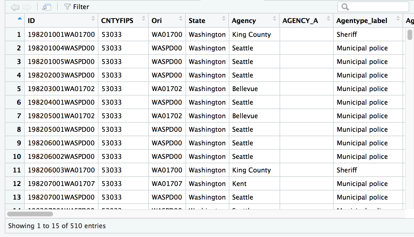
greenway1 <- murders %>%
  filter(State=="Washington" & name_of_county=="King") %>%
  filter(Year >=1982 & Year <=2001) %>%
  filter(VicSex_label=="Female")
View(greenway1)
Alright, we’ve narrowed it down to 510 cases by filtering with “king” county and “Washington” state. We set it between 1982 and 2001 and looked for female victims.
How many of those were strangled? Is there a distinction for that? What types of weapons are labeled by officials?
murders %>%
  select(Weapon_label) %>%
  unique()
## Weapon_label
## 1 Knife or cutting instrument
## 2 Shotgun
## 5 Strangulation - hanging
## 6 Rifle
## 7 Handgun - pistol, revolver, etc
## 41 Personal weapons, includes beating
## 49 Fire
## 54 Other or type unknown
## 69 Firearm, type not stated
## 85 Asphyxiation - includes death by gas
## 89 Narcotics or drugs, sleeping pills
## 101 Blunt object - hammer, club, etc
## 495 Drowning
## 550 Pushed or thrown out window
## 1063 Other gun
## 1099 Poison - does not include gas
## 1708 ExplosivesSo what fits Ridgeway’s methods?
Maybe “Strangulation - hanging” and “Other or type unknown”
greenway2 <- greenway1 %>%
  filter(Weapon_label=="Strangulation - hanging" |
           Weapon_label=="Other or type unknown")
View(greenway2)
Well, that narrowed it down.
Now there are 116 cases.
What were the circumstances for these murders? Can we narrow it down to outdoors?
greenway2 %>%
  group_by(Circumstance_label) %>%
  count() %>%
  arrange(desc(n))
## # A tibble: 13 x 2
## # Groups: Circumstance_label [13]
## Circumstance_label n
## <fct> <int>
## 1 Circumstances undetermined 81
## 2 Other 12
## 3 Rape 4
## 4 Other arguments 4
## 5 Robbery 3
## 6 Other sex offense 3
## 7 Burglary 2
## 8 Argument over money or property 2
## 9 Arson 1
## 10 Narcotic drug laws 1
## 11 Other - not specified 1
## 12 Lovers triangle 1
## 13 All other manslaughter by negligence 1No, it doesn’t appear that’s an option. Only “Circumstances undetermined” and “Other” which are vague.
greenway2 %>%
  group_by(Solved_label) %>%
  summarize(total=n()) %>%
  mutate(percent=round(total/sum(total)*100,2))
## # A tibble: 2 x 3
## Solved_label total percent
## <fct> <int> <dbl>
## 1 No 84 72.4
## 2 Yes 32 27.6We should be clear that there’s no way to tell with this data set that the filtered data we’ve sliced out are all victims of Gary Ridgway. That would involve looking up the case files for each victim or researching the evidence presented at his trial. Still there’s a decent chance based on his confession that some of the victims were listed above.
Mindhunter
Put yourself in the mindset of a detective or criminal profiler.
Can you reverse engineer the process of narrowing down the list of victims and apply it to the data set to surface areas where a serial killer might be murdering with impunity?
What’s the list of patterns you could wrangle the data for?
- Areas with low rates of homicide clearances
- Murders span years, even decades
- Victims are similar in gender
- Method of killing is often repeated
The algorithm
Thomas Hargrove noticed these patterns as a journalist and developed an algorithm that would locate these clusters of murders that showed these signs.
Here it is as it’s programmed in SPSS. You’ll notice that the syntax is reminiscent to what we’ve worked with.
Let’s translate that into R and, specifically, dplyr.
- Case status
- Solved: 0 | Unsolved: 1
- dplyr verb:
mutate()andcase_when()
- Gender of victim
- Male:* 1 | Female: 2 | Unknown:
- dplyr verb:
mutate()andcase_when()
- Creating clustering number
- Counties and MSA
- gender
- weapon value assigned by factor
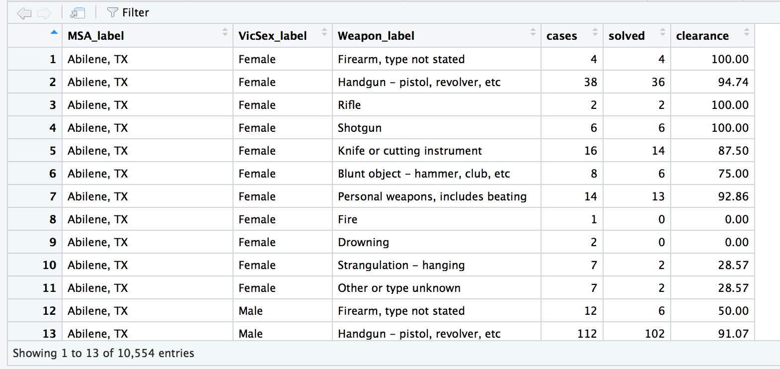
msagrp <- murders %>%
  mutate(solved_num = ifelse(Solved_label=="Yes", 1, 0)) %>%
  group_by(MSA_label, VicSex_label, Weapon_label) %>%
  summarize(cases=n(), solved=sum(solved_num)) %>%
  mutate(clearance=round(solved/cases*100,2))
View(msagrp)
Alright, we have more than 10,000 clusters.
Hargrove says we can filter it further.
Look for female victims, and where clearance rates are less than 33 percent. And where there is more than one victim.
msagrp_filtered <- msagrp %>%
  filter(VicSex_label=="Female" & clearance <= 33 & cases > 1)
datatable(msagrp_filtered)
We have narrowed down 10,000 clusters to 99.
Let’s change the scope and apply what we did to MSAs to Counties.
Why is this distinction important? Well, Metro Statistical Areas consists of at least one county– sometimes whole counties or pieces of it.
Counties are so large that they’re often covered by multiple agencies like town police departments and state police and sheriff’s deputies focusing on different jurisdictions. These things vary but it’s important to note that counties and MSAs– these are just different ways to bin or categorize the data.
Serial killers aren’t limited to by their geography, so it’s important to be flexible with the scope.
countygrp <- murders %>%
  mutate(solved_num = ifelse(Solved_label=="Yes", 1, 0)) %>%
  group_by(county_state, VicSex_label, Weapon_label) %>%
  summarize(cases=n(), solved=sum(solved_num)) %>%
  mutate(clearance=round(solved/cases*100,2)) %>%
  filter(VicSex_label=="Female" & clearance <= 33 & cases > 1) %>%
  arrange(desc(cases))

datatable(countygrp)
Alright, we now have 325 clusters.
Go to the search bar and type in “King, WA”
Cases: 108. Solved: 31. Clearance: 28.7.
Ridgeway’s 75-80 victims are probably among those.
Chilling.
Expanding the scope of the search
Now that we have the basics of this “algorithm” down (it’s basically an illuminating way of grouping and wrangling data), we can add more customization.
We don’t have exclude the genders of men and unknown.
We can limit the scope to the latest 10 years of data.
All by adding or adjusting filters.
countygrp2 <- murders %>%
  # year filter here | remember ":" stands for "through", so 2006:2016 is 2006 2007 2008 etc
  filter(Year %in% 2006:2016) %>%
  mutate(solved_num = ifelse(Solved_label=="Yes", 1, 0)) %>%
  group_by(county_state, VicSex_label, Weapon_label) %>%
  summarize(cases=n(), solved=sum(solved_num)) %>%
  mutate(clearance=round(solved/cases*100,2)) %>%
  filter(clearance <= 33 & cases > 1) %>%
  arrange(desc(cases))

datatable(countygrp2)
Do you think a killer might be targeting a specific age group?
You could filter the age like we did with years or we could create age categories with the data.
Categorical data has been very useful so far. We can turn a continuous variable like age into a categorical variable by dividing it into bins.
We can use case_when() with mutate() from the dplyr package.
Let’s go back to the murders data frame to add this new variable: age_group.
Then we’ll re-run code we created before with that new grouping variable.
Remember, the “:” stand for through. So 0:14 means 0 through 14.
murders <- mutate(murders,
                  age_group=case_when(
                  VicAge %in% 0:14 ~ "0-14",
                  VicAge %in% 15:19 ~ "15-19",
                  VicAge %in% 20:50 ~ "20-50",
                  VicAge %in% 51:99 ~ "51-99",
                  TRUE ~ "Unknown"))

countygrp3 <- murders %>%
  filter(Year %in% 2006:2016) %>%
  mutate(solved_num = ifelse(Solved_label=="Yes", 1, 0)) %>%
  group_by(county_state, VicSex_label, age_group, Weapon_label) %>%
  summarize(cases=n(), solved=sum(solved_num)) %>%
  mutate(clearance=round(solved/cases*100,2)) %>%
  filter(VicSex_label=="Female" & clearance <= 33 & cases > 1) %>%
  arrange(desc(cases))

datatable(countygrp3)
Well done.
I hope this was instrumental in showing you how to approach data to discover insights.
Happy hunting.
© Copyright 2018, Andrew Ba Tran