More R Markdown

Let’s create some R Markdown files.

Make sure your working directory is set.

If you’re not working with the learn-chapter-6-master folder you downloaded with usethis, download your files to a folder called data.

If you get lost, the .Rmd files can be found in the lesson repo.

We’ll start out by generating a report with Boston city payroll data.

Datatables

  1. Create a new R Markdown file and call it Chunk 1.
    • Leave author blank for these exercises

The top of your file (currently called Untitled 1) should look like this:

---
title: "Chunk 1"
output: html_document
---

and then that will be followed by the dummy code.

Delete everything beneath the YAML code.

Replace it with this code:

```{r loading}
# load packages
library(tidyverse)
# Loading the Boston city payroll
payroll <- read_csv("data/bostonpayroll2013.csv")
```
Let's look at the data in R Markdown with a package called [`DT`](https://rstudio.github.io/DT/) that uses the Datatables [jquery library](https://datatables.net/).
```{r display_data}
library(DT)
datatable(payroll)
```
view raw chunk 1 hosted with ❤ by GitHub

Save the file as 01_chunk.Rmd and click the knit button.

Note that you need to save this in learn-chapter-6-master not (as you might have gotten into the habit of doing learn-chapter-6-master/more_rmarkdown

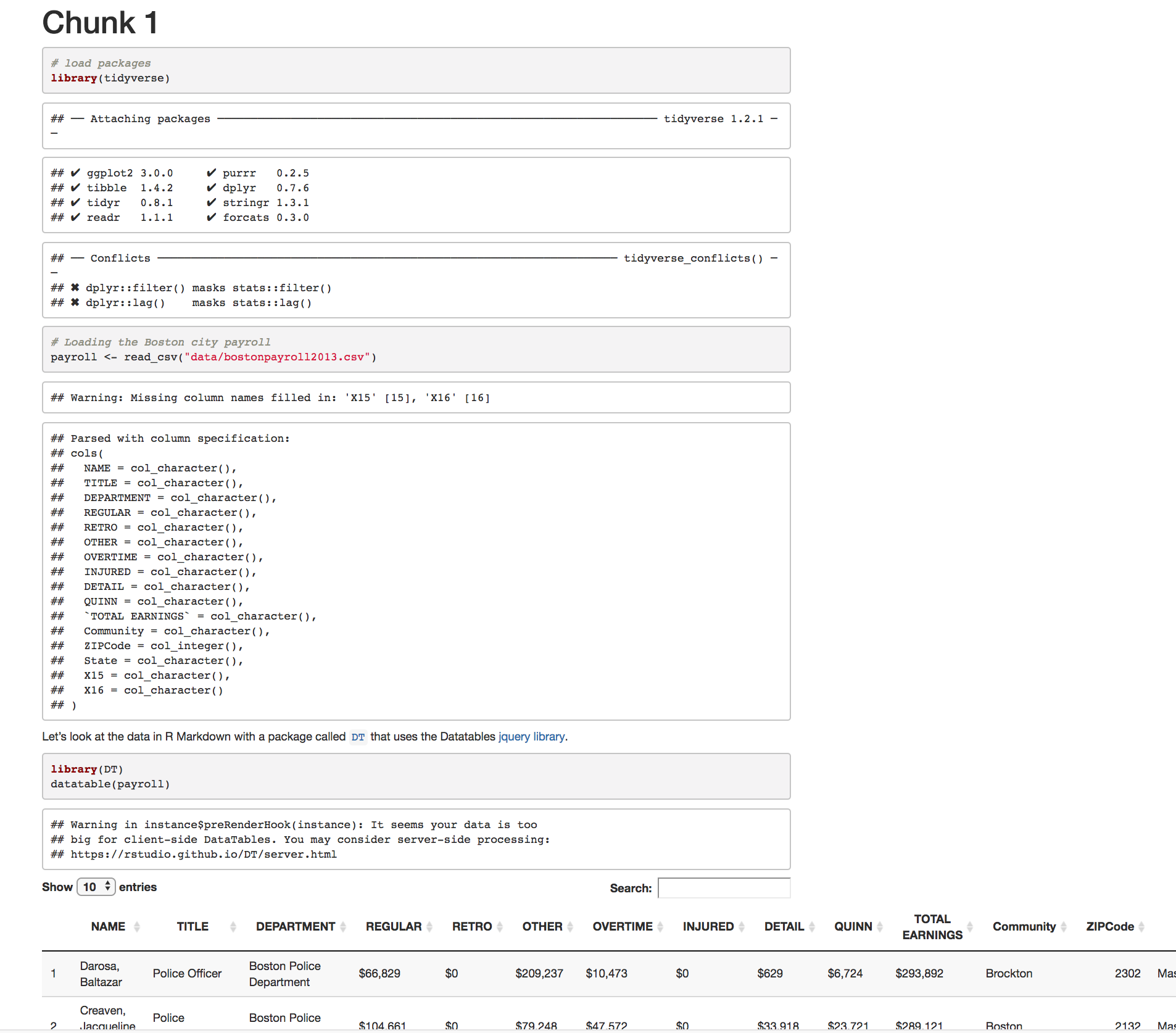
Yikes, okay, that’s way too much.

Hide warnings, messages

We can hide those console messages adding warning=F and message=F by the R code chunk labels.

Create a new R Markdown file and call it Chunk 2.

Type the code in below.

The new code can be found on lines 6 and 16.

---
title: "Chunk 2"
output: html_document
---
```{r loading, warning=F, message=F}
# load packages
library(tidyverse)
# Loading the Boston city payroll
payroll <- read_csv("data/bostonpayroll2013.csv")
```
Let's look at the data in R Markdown with a new package called [`DT`](https://rstudio.github.io/DT/) that uses the Datatables [jquery library](https://datatables.net/).
```{r display_data, warning=F}
library(DT)
datatable(payroll)
```
view raw chunk 2 hosted with ❤ by GitHub

Save the file as 02_chunk.Rmd and click the knit button.

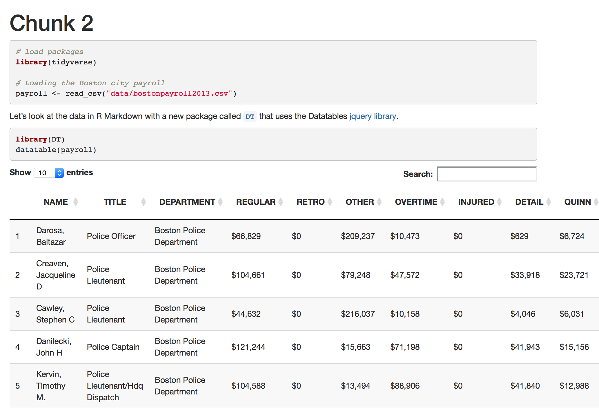
Now that’s much more readable and gets to the data quicker.
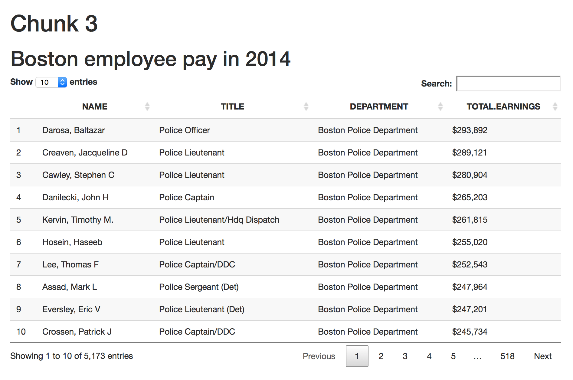
Hide code

If the person you’re sharing this with has no interest in the code and only the quick results, use echo=F to hide the chunk of code and just display the output. It’s on line 8.

We’ll also narrow down the variables selected so the table isn’t way too wide.

Create a new R Markdown file and call it Chunk 3.

Type the code in below.

The new code can be found on 8 and 17.

---
title: "Chunk 3"
output: html_document
---
# Boston employee pay in 2014
```{r loading, warning=F, message=F, echo=F}
# load packages
library(tidyverse)
# Loading the Boston city payroll
payroll <- read_csv("data/bostonpayroll2013.csv")
payroll_total <- select(payroll, NAME, TITLE, DEPARTMENT, TOTAL.EARNINGS)
```
```{r display_data, warning=F, message=F, echo=F}
library(DT)
datatable(payroll_total)
```
view raw Chunk 3 hosted with ❤ by GitHub

Save the file as 03_chunk.Rmd and click the knit button.

Inline R code

Embed lines of R code within the markdown narrative with

Create a new R Markdown file and call it Chunk 4.

Type the code in below.

The new code can be found on line 29 and 31.

---
title: "Chunk 4"
output: html_document
---
```{r loading, warning=F, message=F, echo=F}
# load packages
library(tidyverse)
# Loading the Boston city payroll
payroll <- read_csv("data/bostonpayroll2013.csv")
# Cleaning up column names
colnames(payroll) <- make.names(colnames(payroll))
# Cleaning out dollar signs and commas so it'll convert to numbers correctly
payroll$TOTAL.EARNINGS <- gsub("\\$", "", payroll$TOTAL.EARNINGS)
payroll$TOTAL.EARNINGS <- gsub(",", "", payroll$TOTAL.EARNINGS)
payroll$TOTAL.EARNINGS <- as.numeric(payroll$TOTAL.EARNINGS)
# Narrowing down the scope of the data
payroll_total <- select(payroll, NAME, TITLE, DEPARTMENT, TOTAL.EARNINGS)
most_pay <- payroll_total %>%
arrange(desc(TOTAL.EARNINGS)) %>%
head(1)
```
The Boston city employee who was paid the most in 2014 was a `r most_pay$TITLE` at `r most_pay$DEPARTMENT`.
This person made $`r prettyNum(most_pay$TOTAL.EARNINGS,big.mark=",",scientific=FALSE)`.
```{r display_data, warning=F, message=F, echo=F}
library(DT)
datatable(payroll_total)
```
view raw Chunk 4 hosted with ❤ by GitHub

Save the file as 04_chunk.Rmd and click the knit button.

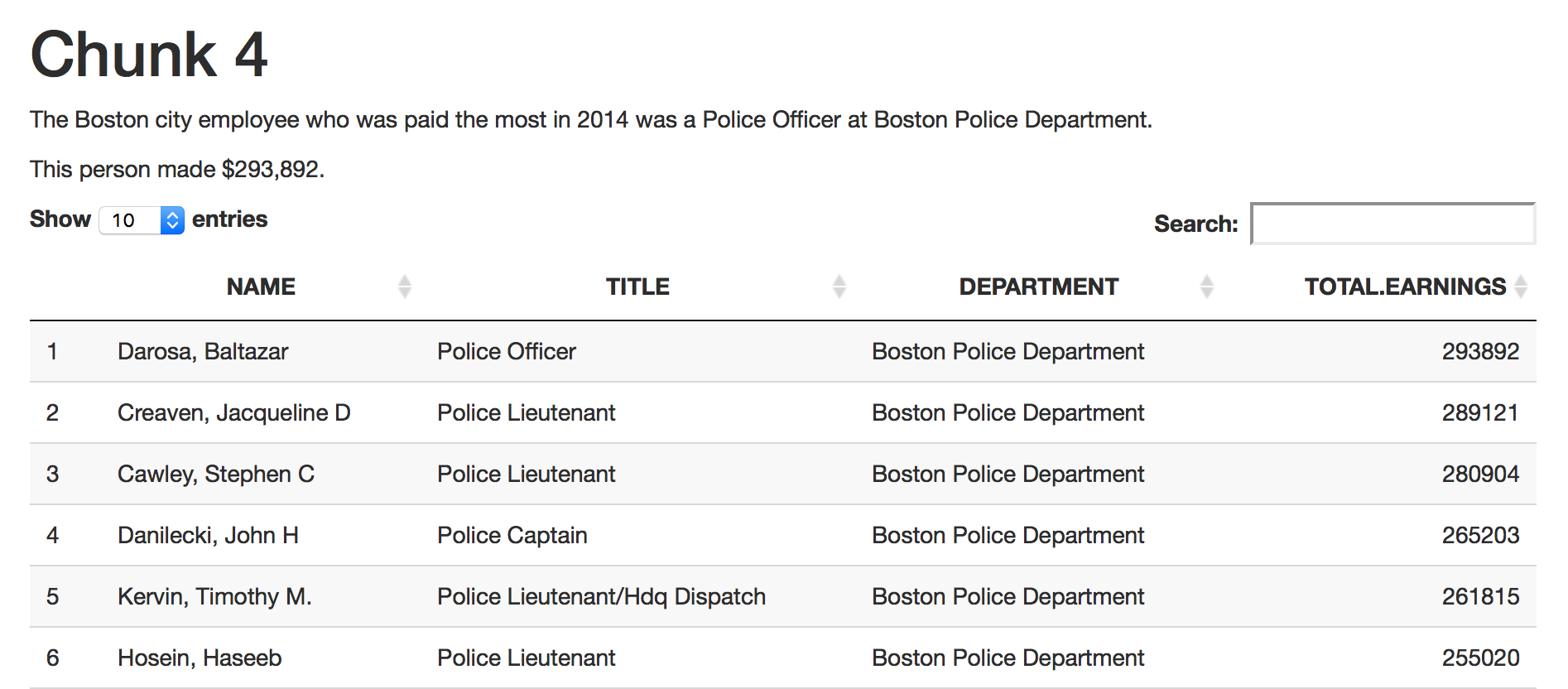
This type of self-generating analysis is important because if you get the next year of payroll data, running this report will sub in the new city employee who makes the most money automatically.

Pretty tables

Make pretty tables with the knitr package and the kable() function.

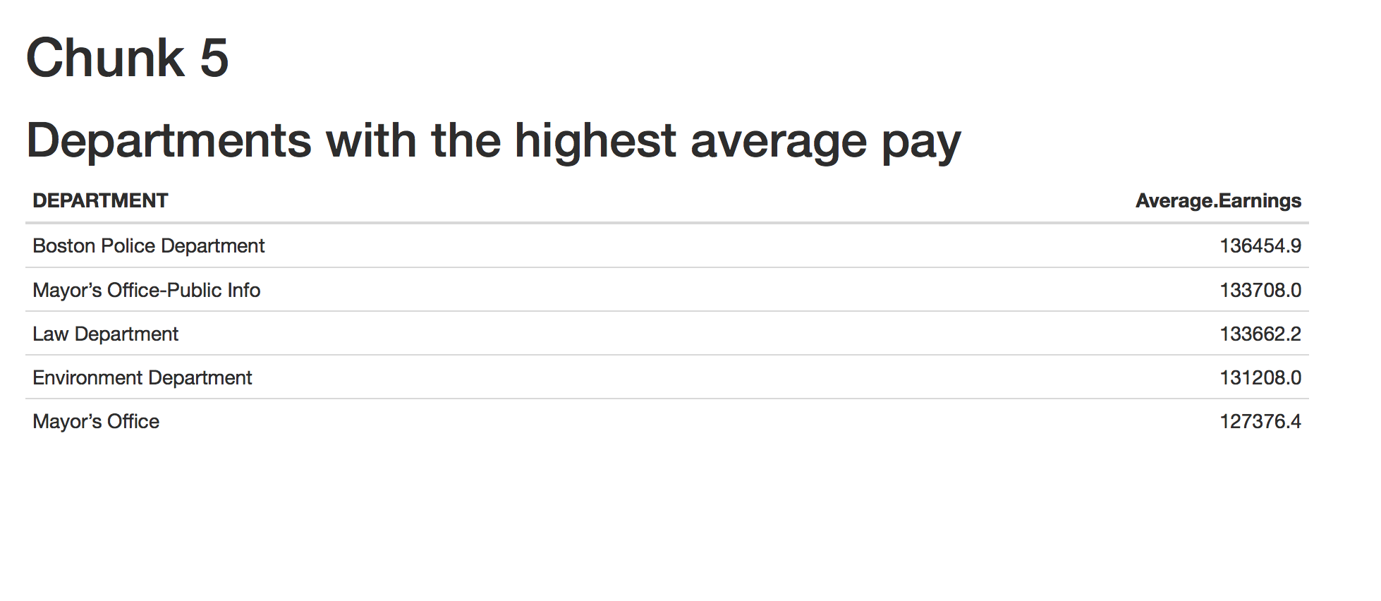
Create a new R Markdown file and call it Chunk 5.

Type the code in below.

The new code can be found all the way down on line 60 and 61.

---
title: "Chunk 5"
output: html_document
---
# Departments with the highest average pay
```{r loading, warning=F, message=F, echo=F}
# load packages
library(tidyverse)
# Loading the Boston city payroll
payroll <- read_csv("data/bostonpayroll2013.csv")
```
```{r cleaning_data, warning=F, echo=F}
colnames(payroll) <- make.names(colnames(payroll))
payroll$REGULAR <- gsub("\\$", "", payroll$REGULAR)
payroll$REGULAR <- gsub(",", "", payroll$REGULAR)
payroll$REGULAR <- as.numeric(payroll$REGULAR)
payroll$RETRO <- gsub("\\$", "", payroll$RETRO)
payroll$RETRO <- gsub(",", "", payroll$RETRO)
payroll$RETRO <- as.numeric(payroll$RETRO)
payroll$OTHER <- gsub("\\$", "", payroll$OTHER)
payroll$OTHER <- gsub(",", "", payroll$OTHER)
payroll$OTHER <- as.numeric(payroll$OTHER)
payroll$OTHER <- gsub("\\$", "", payroll$OTHER)
payroll$OTHER <- gsub(",", "", payroll$OTHER)
payroll$OTHER <- as.numeric(payroll$OTHER)
payroll$OVERTIME <- gsub("\\$", "", payroll$OVERTIME)
payroll$OVERTIME <- gsub(",", "", payroll$OVERTIME)
payroll$OVERTIME <- as.numeric(payroll$OVERTIME)
payroll$INJURED <- gsub("\\$", "", payroll$INJURED)
payroll$INJURED <- gsub(",", "", payroll$INJURED)
payroll$INJURED <- as.numeric(payroll$INJURED)
payroll$DETAIL <- gsub("\\$", "", payroll$DETAIL)
payroll$DETAIL <- gsub(",", "", payroll$DETAIL)
payroll$DETAIL <- as.numeric(payroll$DETAIL)
payroll$QUINN <- gsub("\\$", "", payroll$QUINN)
payroll$QUINN <- gsub(",", "", payroll$QUINN)
payroll$QUINN <- as.numeric(payroll$QUINN)
payroll$TOTAL.EARNINGS <- gsub("\\$", "", payroll$TOTAL.EARNINGS)
payroll$TOTAL.EARNINGS <- gsub(",", "", payroll$TOTAL.EARNINGS)
payroll$TOTAL.EARNINGS <- as.numeric(payroll$TOTAL.EARNINGS)
```
```{r analysis, warning=F, message=F, echo=F}
top5 <- payroll %>%
group_by(DEPARTMENT) %>%
summarize(Average.Earnings=mean(TOTAL.EARNINGS, na.rm=T)) %>%
arrange(desc(Average.Earnings)) %>%
head(5)
```
```{r table, warning=F, echo=F}
library(knitr)
kable(top5)
```
view raw Chunk 5 hosted with ❤ by GitHub

Save the file as 05_chunk.Rmd and click the knit button.

Change theme and style

Change the appearance and style of the HTML document by changing the theme up top.

Options from the Bootswatch theme library includes:

  • default
  • cerulean
  • journal
  • cosmo

highlights (for the code syntax)

  • tango
  • pygments
  • kate

Create a new R Markdown file and call it Chunk 6.

Type the code in below.

The new code is at the top in the YAML section.

---
title: "Chunk 6"
author: "Andrew"
date: "7/23/2018"
output:
html_document:
theme: united
highlight: espresso
---
```{r loading, warning=F, message=F, echo=F}
# load packages
library(tidyverse)
# Loading the Boston city payroll
payroll <- read_csv("data/bostonpayroll2013.csv")
```
```{r cleaning_data, warning=F, echo=F}
colnames(payroll) <- make.names(colnames(payroll))
payroll$REGULAR <- gsub("\\$", "", payroll$REGULAR)
payroll$REGULAR <- gsub(",", "", payroll$REGULAR)
payroll$REGULAR <- as.numeric(payroll$REGULAR)
payroll$RETRO <- gsub("\\$", "", payroll$RETRO)
payroll$RETRO <- gsub(",", "", payroll$RETRO)
payroll$RETRO <- as.numeric(payroll$RETRO)
payroll$OTHER <- gsub("\\$", "", payroll$OTHER)
payroll$OTHER <- gsub(",", "", payroll$OTHER)
payroll$OTHER <- as.numeric(payroll$OTHER)
payroll$OTHER <- gsub("\\$", "", payroll$OTHER)
payroll$OTHER <- gsub(",", "", payroll$OTHER)
payroll$OTHER <- as.numeric(payroll$OTHER)
payroll$OVERTIME <- gsub("\\$", "", payroll$OVERTIME)
payroll$OVERTIME <- gsub(",", "", payroll$OVERTIME)
payroll$OVERTIME <- as.numeric(payroll$OVERTIME)
payroll$INJURED <- gsub("\\$", "", payroll$INJURED)
payroll$INJURED <- gsub(",", "", payroll$INJURED)
payroll$INJURED <- as.numeric(payroll$INJURED)
payroll$DETAIL <- gsub("\\$", "", payroll$DETAIL)
payroll$DETAIL <- gsub(",", "", payroll$DETAIL)
payroll$DETAIL <- as.numeric(payroll$DETAIL)
payroll$QUINN <- gsub("\\$", "", payroll$QUINN)
payroll$QUINN <- gsub(",", "", payroll$QUINN)
payroll$QUINN <- as.numeric(payroll$QUINN)
payroll$TOTAL.EARNINGS <- gsub("\\$", "", payroll$TOTAL.EARNINGS)
payroll$TOTAL.EARNINGS <- gsub(",", "", payroll$TOTAL.EARNINGS)
payroll$TOTAL.EARNINGS <- as.numeric(payroll$TOTAL.EARNINGS)
```
```{r analysis, warning=F, message=F}
top5 <- payroll %>%
group_by(DEPARTMENT) %>%
summarize(Average.Earnings=mean(TOTAL.EARNINGS, na.rm=T)) %>%
arrange(desc(Average.Earnings)) %>%
head(5)
```
```{r table, warning=F, echo=F}
library(knitr)
kable(top5)
```
view raw Chunk 6 hosted with ❤ by GitHub

Save the file as 06_chunk.Rmd and click the knit button.
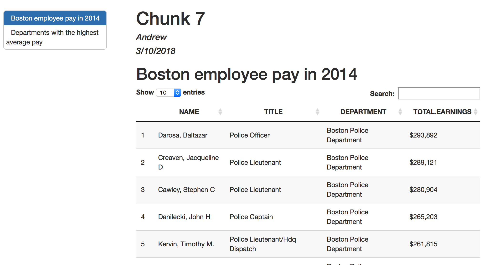
Table of contents

Add a floating table of contents by changing html_document to toc: true and toc_float: true.

Create a new R Markdown file and call it Chunk 7.

Type the code in below.

The new code is at the top in the YAML section.

---
title: "Chunk 7"
author: "Andrew"
date: "3/10/2018"
output:
html_document:
toc: true
toc_float: true
---
# Boston employee pay in 2014
```{r loading, warning=F, message=F, echo=F}
# load packages
library(tidyverse)
# Loading the Boston city payroll
payroll <- read_csv("data/bostonpayroll2013.csv")
colnames(payroll) <- make.names(colnames(payroll))
payroll_total <- select(payroll, NAME, TITLE, DEPARTMENT, TOTAL.EARNINGS)
```
```{r display_data, warning=F, message=F, echo=F}
library(DT)
datatable(payroll_total)
```
# Departments with the highest average pay
```{r cleaning_data, warning=F, echo=F}
payroll$REGULAR <- gsub("\\$", "", payroll$REGULAR)
payroll$REGULAR <- gsub(",", "", payroll$REGULAR)
payroll$REGULAR <- as.numeric(payroll$REGULAR)
payroll$RETRO <- gsub("\\$", "", payroll$RETRO)
payroll$RETRO <- gsub(",", "", payroll$RETRO)
payroll$RETRO <- as.numeric(payroll$RETRO)
payroll$OTHER <- gsub("\\$", "", payroll$OTHER)
payroll$OTHER <- gsub(",", "", payroll$OTHER)
payroll$OTHER <- as.numeric(payroll$OTHER)
payroll$OTHER <- gsub("\\$", "", payroll$OTHER)
payroll$OTHER <- gsub(",", "", payroll$OTHER)
payroll$OTHER <- as.numeric(payroll$OTHER)
payroll$OVERTIME <- gsub("\\$", "", payroll$OVERTIME)
payroll$OVERTIME <- gsub(",", "", payroll$OVERTIME)
payroll$OVERTIME <- as.numeric(payroll$OVERTIME)
payroll$INJURED <- gsub("\\$", "", payroll$INJURED)
payroll$INJURED <- gsub(",", "", payroll$INJURED)
payroll$INJURED <- as.numeric(payroll$INJURED)
payroll$DETAIL <- gsub("\\$", "", payroll$DETAIL)
payroll$DETAIL <- gsub(",", "", payroll$DETAIL)
payroll$DETAIL <- as.numeric(payroll$DETAIL)
payroll$QUINN <- gsub("\\$", "", payroll$QUINN)
payroll$QUINN <- gsub(",", "", payroll$QUINN)
payroll$QUINN <- as.numeric(payroll$QUINN)
payroll$TOTAL.EARNINGS <- gsub("\\$", "", payroll$TOTAL.EARNINGS)
payroll$TOTAL.EARNINGS <- gsub(",", "", payroll$TOTAL.EARNINGS)
payroll$TOTAL.EARNINGS <- as.numeric(payroll$TOTAL.EARNINGS)
```
```{r analysis, warning=F, message=F, echo=F}
top5 <- payroll %>%
group_by(DEPARTMENT) %>%
summarize(Average.Earnings=mean(TOTAL.EARNINGS, na.rm=T)) %>%
arrange(desc(Average.Earnings)) %>%
head(5)
```
```{r table, warning=F, echo=F}
library(knitr)
kable(top5)
```
view raw Chunk 7 hosted with ❤ by GitHub

Save the file as 07_chunk.Rmd and click the knit button.

Next steps?

Exporting as a PDF will require LaTex installed first * Get it from latex-project.org or MacTex

Check out all the features of R Markdown at RStudio

Publish your results to Github pages


© Copyright 2018, Andrew Ba Tran

© Copyright 2018, Andrew Tran