R for Journalists > Spatial analysis > Interactive maps with Leaflet

Interactive maps with Leaflet

Let’s create a locator map like you would when searching for an address on Google Maps.

Sometimes it’s necessary to zoom in or pan around a map for greater comprehension while exploring data spatially.

The Leaflet R package was created by the folks behind RStudio to integrate with the popular opensource JavaScript library.

It’s great for journalists who have little knowledge of JavaScript who want to make interesting interactives using R. And there is excellent documentation if you want to dig deeper into its functionality after this introduction.

Essentially, this package lets you make maps with custom map tiles, markers, polygons, lines, popups, and geojson. Almost any maps you can make in Google Fusion Tables or Carto(DB), you can make in R using the Leaflet package.

# Uncomment and run "install.packages" functions below if you have not yet installed these packages

#install.packages("leaflet")

# IF YOU GET AN ERROR BECAUSE THERE IS NO PACKAGE CALLED httpuv
#install.packages("httpuv")
#install.packages("leaflet")

library(leaflet)




#install.packages("dplyr")
library(dplyr)

Putting a marker on a map

Let’s begin by finding a latitude and longitude to map.

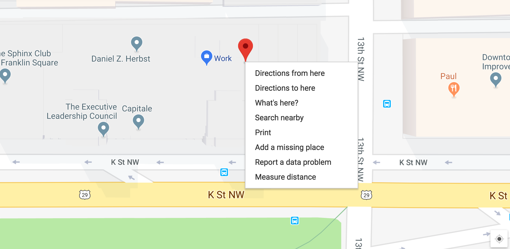
Go to Google Maps and search for any address.

Right click on the map until you get this menu.

Select “What’s here?” and at the bottom copy and paste that latitude and longitude.

Create a map widget by calling the leaflet() function
Add layers (such as features) to the map by using layer functions
- like addTiles, addMarkers, addPolygons
Print the map widget
Customize the view port zoom and center location with setView()

# Insert your latitude and longitude in the code below
# NOTE: Don't get them reversed otherwise you'll end up in the South Pole.

# Initialize and assign m as the leaflet object
m <- leaflet() %>%
# Now add tiles to it
    addTiles() %>%  
# Setting the middle of where the map should be and the zoom level
    setView(lng=-77.030137, lat=38.902986, zoom = 16) %>%
# Now, add a marker with a popup, 
    addMarkers(lng=-77.030137, lat=38.902986, popup="<b>Hello</b><br><a href='https://www.washingtonpost.com'>-Me</a>")

m

Go ahead and click the blue marker.

Explaining the R code

leaflet() initializes the leaflet work space
addTiles() by itself will bring in the default OpenStreetMap tiles
- Here’s a list of free leaflet tiles you can use
- Note: OpenStreetMaps is a wonderful and free open-source service. Their only stipulation for using their tiles is to be sure to credit and link to them in the map.
setView() is pretty self-explanatory but is simpler to implement
addMarkers() with some specific parameters.

Note: The order of commands is important. A view can’t be set unless there are tiles established first.

How to put the map online

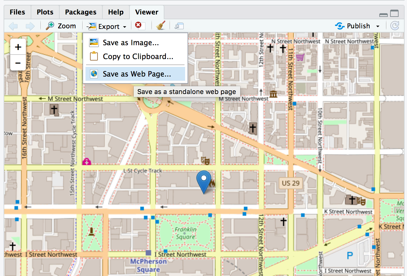
Run the code in your RStudio console and it will appear in your Viewer tab.

Click on Export > Save as Web page.

Export

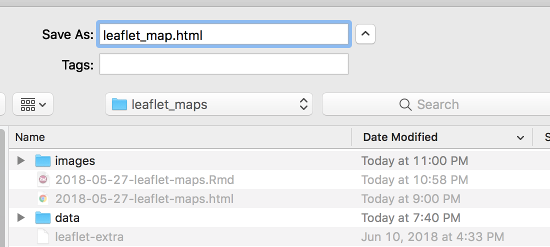
Give it a file name and click save.

Save as

You have the map now as a full screen html file.

File

You can upload the file wherever you like and then iframe to it if you want to embed it into website like the code below.

<iframe src="leaflet_map.html" frameborder="0" width="100%" height="300px"></iframe>

Or you can leave it embedded in an R Markdown file as the raw R code, like I have in this file.

When comparing the size of the HTML files, the R-produced version of the map is larger in size because it is bringing all the JavaScript and CSS inline into the HTML. However, when looking at how much data is actually downloaded to load the map html, the differences aren’t as drastic.

Multiple locations from a csv

Let’s bring in some new data.

library(readr)
dunkin <- read_csv("data/dunkin.csv")

## Parsed with column specification:
## cols(
##   id = col_integer(),
##   address = col_character(),
##   city = col_character(),
##   state = col_character(),
##   zip = col_integer(),
##   country = col_character(),
##   lat = col_double(),
##   lon = col_double(),
##   type = col_character()
## )

glimpse(dunkin)

## Observations: 7,794
## Variables: 9
## $ id      <int> 300176, 300178, 300179, 300202, 300204, 300205, 300208...
## $ address <chr> "1752B Route 9", "99 High St", "17 Railroad Ave", "411...
## $ city    <chr> "Clifton Park", "Danvers", "Rockport", "Holbrook", "Ea...
## $ state   <chr> "NY", "MA", "MA", "NY", "NJ", "MA", "MA", "MA", "MA", ...
## $ zip     <int> 12065, 1923, 1966, 11741, 7018, 2021, 2301, 2188, 2145...
## $ country <chr> "US", "US", "US", "US", "US", "US", "US", "US", "US", ...
## $ lat     <dbl> 42.87174, 42.55958, 42.65634, 40.80692, 40.75238, 42.1...
## $ lon     <dbl> -73.77414, -70.93124, -70.62621, -73.07295, -74.20798,...
## $ type    <chr> "Dunkin Donuts", "Dunkin Donuts", "Dunkin Donuts", "Du...

We’ve imported nearly 8,000 rows of Dunkin’ Donuts store location data.

Let’s limit it a bit because 8,000 dots on a slippy map is taxing on a browser.

# Pick a state, any state.
# I'll use Massachusetts here because that's where Dunkin started

dd_state <- dunkin %>% 
  filter(state=="MA")

Let’s make a map with a new tile set. Instead of leaving addTiles() empty, we’ll pass on some new data to some third-party tiles with the addProviderTiles() function. Check out all the neat tile options.

Some options to use with addCircles includes the data to pull in for popup and color, which we’ve made bright orange. We’ve also set radius and weight and fillOpacity.

If we wanted to change the radius of the circle based on some data point, you could replace 40 with some column with numeric values in it.

m <- leaflet(dd_state) %>% addProviderTiles(providers$CartoDB.DarkMatter) %>% 
  setView(-71.931180, 42.385453, zoom = 7) %>% 
  addCircles(~lon, ~lat, popup=dunkin$type, weight = 3, radius=40, 
                 color="#ffa500", stroke = TRUE, fillOpacity = 0.8) 
m

Why stop there?

Let’s bring in some competition.

starbucks <- read_csv("data/starbucks.csv")

## Parsed with column specification:
## cols(
##   `Store Number` = col_integer(),
##   `Store Name` = col_character(),
##   Address = col_character(),
##   `Address Line2` = col_character(),
##   City = col_character(),
##   Province = col_character(),
##   `Postal Code` = col_character(),
##   `Phone Number` = col_character(),
##   `Store Hours` = col_character(),
##   `Wireless?` = col_character(),
##   lat = col_double(),
##   lon = col_double(),
##   type = col_character()
## )

glimpse(starbucks)

## Observations: 11,135
## Variables: 13
## $ `Store Number`  <int> 79797, 79796, 79795, 79794, 79793, 79789, 7978...
## $ `Store Name`    <chr> "Dominick's-Chicago #1100", "Safeway - Chandle...
## $ Address         <chr> "3145 S Ashland Ave", "1159 W Chandler Blvd", ...
## $ `Address Line2` <chr> NA, NA, NA, NA, NA, NA, NA, NA, NA, NA, NA, NA...
## $ City            <chr> "Chicago", "Chandler", "Mansfield", "Bothell",...
## $ Province        <chr> "IL", "AZ", "TX", "WA", "WA", "CA", "CA", "SC"...
## $ `Postal Code`   <chr> "60608-6251", "85224-5202", "76063-2602", "980...
## $ `Phone Number`  <chr> "773-247-2633", "480-726-7776", "817-453-6770"...
## $ `Store Hours`   <chr> "Mon: 6:00 AM-8:00 PM Tue: 6:00 AM-8:00 PM Wed...
## $ `Wireless?`     <chr> NA, NA, NA, "Wireless Hotspot", "Wireless Hots...
## $ lat             <dbl> 41.83619, 33.30424, 32.58408, 47.78450, 47.269...
## $ lon             <dbl> -87.66409, -111.86316, -97.13298, -122.21282, ...
## $ type            <chr> "Starbucks", "Starbucks", "Starbucks", "Starbu...

We should filter it so it’s only the state for which we already filtered for Dunkin data.

sb_state <- starbucks %>% 
  filter(Province=="MA")

The data is structured a bit differently, but at least it has type and location data.

Also, let’s switch from addCircles to addCircleMarkers.

# isolating just the 3 columns we're interested in-- type, lat, and lon
sb_loc <- select(sb_state, type, lat, lon)
dd_loc <- select(dd_state, type, lat, lon)

# joining the two data frames together
ddsb <- rbind(sb_loc, dd_loc)

# creating a coffee color palette

cof <- colorFactor(c("#ffa500", "#13ED3F"), domain=c("Dunkin Donuts", "Starbucks"))
# mapping based on type
m <- leaflet(ddsb) %>% 
  addProviderTiles(providers$CartoDB.DarkMatter) %>% 
  setView(-71.931180, 42.385453, zoom = 7) %>% 
  addCircleMarkers(~lon, ~lat, popup=ddsb$type, weight = 3, radius=4, 
                 color=~cof(type), stroke = F, fillOpacity = 0.5) 
m

Play around with the slippy map. Interesting, right?

The file size is only 1.3 m even though there are more than 1,300 points on the map.

Still, that’s a lot of points to process. I don’t recommend more.

Add a legend

Let’s add a legend with the function addLegend() and options for where to place it and colors and labels.

m <- leaflet(ddsb)  %>% 
  addProviderTiles(providers$CartoDB.DarkMatter) %>% 
  setView(-71.931180, 42.385453, zoom = 7) %>% 
  addCircleMarkers(~lon, ~lat, popup=ddsb$type, weight = 3, radius=4, 
                 color=~cof(type), stroke = F, fillOpacity = 0.5)  %>%
  addLegend("bottomright", colors= c("#ffa500", "#13ED3F"), labels=c("Dunkin'", "Starbucks"), title="Coffee places") 

m