Introduction to R
Working directories
Your working directory is the folder on your computer in which you are currently working. When you ask R to open a certain file, it will look in the working directory for this file, and when you tell R to save a data file or figure, it will save it in the working directory.
Before you start working, please set your working directory tow here all your data and script files are or should be stored.
Type in the command window:
# On a mac, it'd look like this
setwd("~/projects/learn-r-journalism")

# On a pc, it might look like this
setwd("C:/Documents/learn-r-journalism")
Make sure that slashes are forward slashes and that you don’t forget the quotation marks. R is also case sensitive, so make sure you write cpitals where necessary
Within RStudio, you can also set the working directory via the menu Tools > Set Working Directory

Libraries
R can do many statistical and data analyses.
They are organized in so-called packages or libraries. With the standard installation (known as base), most common packages are installed.
To get a list of all installed packages, go to the packages window or type library() in the console window. If the box in front of the package name is ticked, the package is loaded (activated) and can be used.
There are many more packages available on the R website. If you want to install and use a package (for example, the packaged called “geometry”) you should:
- Install the package: click
install packagesin the packages window and typegeometryor typeinstall.packages("geometry")in the command window. - Load the package: Check box in front of
gemoetryor typelibrary("geometry")in the command window.
Examples of R commands
Calculator
R can be used as a calculator.
Just type an equation in the command window after the >
10^2 + 26## [1] 126Workspace
You can give numbers a name.
By doing so, they become so-called variables which can be used later.
a <- 4
a
## [1] 4You can do calculations with a now.
a*5## [1] 20If you specify a again, it will forget what value you had before because you did not assign it to anything.
a## [1] 4You can also assign a value to a using the old one
a <- a + 10
a
## [1] 14To remove all variables from R’s memory, type
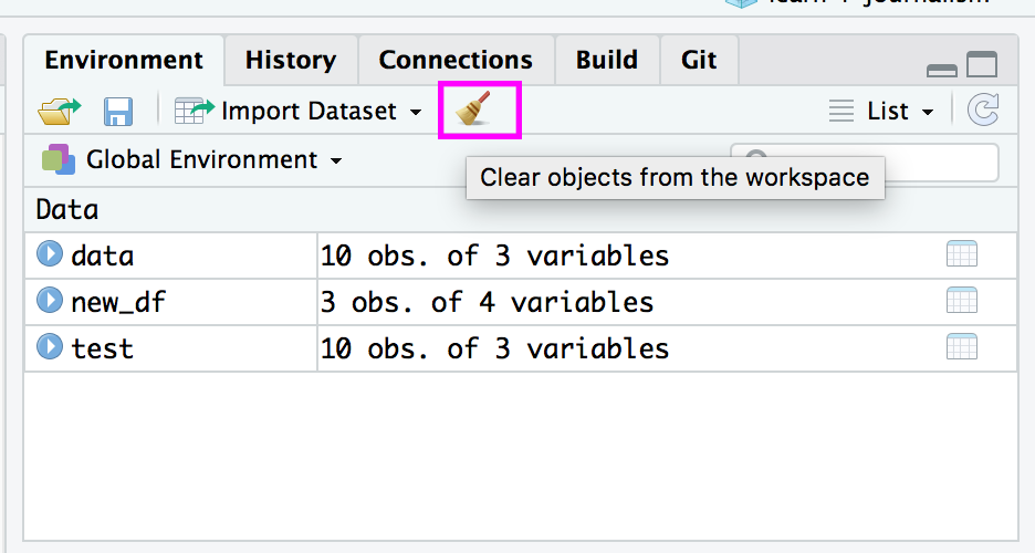
rm(list=ls())or click the “clear all” broom button in the workspace window.
Scalars, vectors, and matrices
Like in many other programs, R organizes numbers in scalars (a single number 0-dimensional), vectors (a row of numbers, also called arrays - `-dimensional) and matrices (like a table - 2-dimensional).
The a you defined was scalar.
To define a vector with the numbers 3,4, and 5, you need the function c() which is short for concatenate (or paste together).
b=c(3,4,5)
b
## [1] 3 4 5Functions
If you would like to compute the mean of all the elements in the vector b from the example above, you could type
(3+4+5)/3## [1] 4But when the vector is very long, this is very boring and time-consuming work.
Thi is why things you do often are automated in so-called functions. Some functions are standard in R or in one of the pakages. You can also program your own functions.
When you use a function to compute a mean, you’ll type
mean(x=b)## [1] 4Whithin the brackets you specify the arguments.
Arguments give extra information to the function. In this case, the argument x says of which set of numbers (vector) the mean should computed (namely of b).
Sometimes the name of the argument is not necessary:
mean(b)## [1] 4Also works.
Plots
R can make simple graphics right away.
# rnorm() is a base function that creates random samples from a random distribution

x <- rnorm(100)

# plot() is a base function that charts

plot(x)
- In the first line, 100 random numbers are assigned to the variable x, which becomes a vector by this operation.
- In the second line, all these values are plotted in the plot window.
Scripts
R is an interpreter that uses a command line based environment.
This means that you have to type commands, rather than use the mouse and menus.
This has the advantage that you do not always have to retype commands.
You can store yoru commands in files, the so-called scripts. These scripts have typically file names with the extension .R as in script.R.
You can open an editor window to edit these files by clicking File > New or File > Open file…
You can run (send to the console window) part of the code by selecting lines and pressing CTRL+ENTER or CMD+ENTER or click the Run button at the top of the script editor window. If you do not select anything, R will run the line your cursor is on.
You can always run the whole script with the function source()
For example, to run the entire saved script.R if it’s in the root directory of the working directory, type
source("script.R")You can also click Run all in the editor window or type CTRL+SHIFT+S or CMD+SHIFT+S
Not available data
When you work with real data, you will encounter missing values because instrumentation failed or because you didn’t want to measure in the weekend.
When a data is not available, you write NA instead of a number.
j <- c(1,2,NA)Computing statistics of incomplete data sets is strictly not possible.
maybe the largest value occured during the weekend when you didn’t measure. Therefore, R will say that it doesn’t know what the largest value of j is
max(j)## [1] NAIf you don’t mind about the missing data and want to compute the statistics anyway, you can add the argument na.rm=TRUE (Should I remove the NAs? Yes)
max(j, na.rm=T)## [1] 2NAs will also affect any sort of math if you’re not careful
sum(j)## [1] NA# compared to
sum(j, na.rm=T)## [1] 3Classes
We’ve been working so far with numbers.
But sometimes data we work with can be specified as something else, like characters and strings or boolean values like TRUE or FALSE or dates.
Characters
m <- "apples"
m
## [1] "apples"To tell R that something is a character string, you should type the text between apostrophes, otherwise R will start looking for a defined veriable with the same name.
n <- pears## Error in eval(expr, envir, enclos): object 'pears' not foundYou can’t do math with characters.
m + 2## Error in m + 2: non-numeric argument to binary operatorDates
Dates and times are complicated.
R has to know that 3 o’clock comes after 2:59 and that February has 29 days in some years.
The base way to tell R that something is a date-time combination is with the function strptime()
date1 <- strptime(c("20100225230000", "20100226000000", "20100226010000"), format="%Y%m%d%H%M%S")
date1
## [1] "2010-02-25 23:00:00 EST" "2010-02-26 00:00:00 EST"
## [3] "2010-02-26 01:00:00 EST"A vector is created with c() and the numbers between the quotation marks are strings, because that’s what the strptim() function requires.
That’s followed by the argument format that defines how the chracter string should be read. In this instance, the year is denoted first (%Y), then the month (%M) and second (%S). You don’t have to specify all of them, as long as the format corresponds to the character string.
In this course, we’ll be using a less messy way to deal with dates using the package lubridate.
# If you don't currently have the lubridate package installed, uncomment the line below and run it

# install.packages("lubridate")

library(lubridate)
##
## Attaching package: 'lubridate'## The following object is masked from 'package:base':
##
## datedate1 <- ymd_hms(c("20100225230000", "20100226000000", "20100226010000"))Factors
Complicated.
They’re categorical variables that are useful for statisticians with plots and regression analysis.
For example, Race might be input as “White”, “Black”, and “Hispanic”
When importing that data in from a spreadsheet, R will most often interpret it as a Factor.
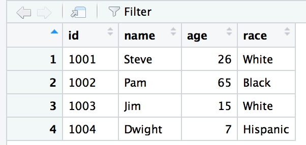
Let’s take a look at the structure behind a dataframe I’ve included, called sample_df
str(sample_df)## 'data.frame': 4 obs. of 4 variables:
## $ id : Factor w/ 4 levels "1001","1002",..: 1 2 3 4
## $ name: chr "Steve" "Pam" "Jim" "Dwight"
## $ age : num 26 65 15 7
## $ race: Factor w/ 3 levels "Black","Hispanic",..: 3 1 3 2R sees that the Race column is a factor variable with three levels.
levels(sample_df$race)## [1] "Black" "Hispanic" "White"This means that R groups statistics by these levels.
summary(sample_df$race)## Black Hispanic White
## 1 1 2Internally, R stores the integer values 1, 2, and 3, and maps the character strings in alphabetical order to these values. 1=Black, 2=Hispanic, and 3=White.
Why is this important to know?
Journalists are less concerned by factors and will often find themselves converting factors to strings and characters. But when you reach the point that you are wanting to create models and linear regressions then you’ll be happy that it’s an option.
Most odd quirks when it comes to R can be traced back to the fact that R was created by and for statisticians. R has grown a lot since then and the community has helped make it evolve to handle data the way we are more used to. But some habits die hard and are ingrained.
Integers & Numbers
Self-explanatory. Saves as whole numbers or nummbers.
Converting between the different types
Here’s a warning.
- You can convert factors into strings.
sample_df$race## [1] White Black White Hispanic
## Levels: Black Hispanic Whiteas.character(sample_df$race)## [1] "White" "Black" "White" "Hispanic"- You can convert strings into factors
sample_df$name## [1] "Steve" "Pam" "Jim" "Dwight"factor(sample_df$name)## [1] Steve Pam Jim Dwight
## Levels: Dwight Jim Pam Steve- You cannot convert factors into numbers.
sample_df$id## [1] 1001 1002 1003 1004
## Levels: 1001 1002 1003 1004as.numeric(sample_df$id)## [1] 1 2 3 4Because R stores Factors as Integer values.
You must convert factors into characters first before converting it to numbers.
So you can nest it.
sample_df$id## [1] 1001 1002 1003 1004
## Levels: 1001 1002 1003 1004as.numeric(as.character(sample_df$id))## [1] 1001 1002 1003 1004Functions
You can also save code you’ve written that simplifies your process into a function.
percent_change <- function(first_number, second_number) {
  pc <- (second_number-first_number)/first_number*100
  return(pc)
}

percent_change(100,150)
## [1] 50This is what’s happening in the code above:
- percent_change is the name of the function, and assigned to it is the function
function() - Two variables are necessary to be passed to this function, first_number and second_number
- A new object
pcis created using some math calculating percent change from the two variables passed to it - the function
return()assigns the result of the math topercent_changefrom the first line
Build enough functions and you can save them as your own package.
The important thing about functions is that they’re programmed by humans.
I constructed this function because that’s how I know that I’ll only include two inputs and that each one will be numeric and that they’ll be in order of first then second.
If you’re working in R and a function you’re using is giving an error, it most likely means there’s something wrong with one or more of the variables you’re passing to the function.
Here’s what happens when I pass a string to my percent_change() function.
percent_change("what", "happens")## Error in second_number - first_number: non-numeric argument to binary operatorSometimes really great R programmers will anticipate errors and catch bad inputs and try to output helpful suggestions instead of a generic error.
This particular error isn’t very explicit. It needs to be interpreted but you know that the function needs numbers to work correctly.
New users might not know that intuitively.
And that’s how you’re going to feel when functions you run don’t work.
You’ll have to Google the error or peek into code to see if you can see what it expects and how it might break down thanks to what you’ve passed it.
And it won’t be entirely your fault.
When we’re coding and sharing it for others we can’t anticipate all the ways in which others might want to use it in the future.
Shoot the function writer a message or if you wrote the package, welcome feedback from others.
This is what makes participating in the R community so great. We just want to do better.