R for Journalists > Importing/Exporting data > SPSS data

SPSS data

SPSS is similar to Excel in that it’s proprietary software that stores data in a very specific format and provides a graphical interface useful for even deeper analysis.

It stands for Statistical Package for the Social Sciences and is owned by IBM. It’s also very expensive and usually only large businesses or organizations own licenses.

But it’s possible to bring in data saved from SPSS into R.

In this example, we’ll be working with case-level data from the FBI’s Supplementary Homicide Report. It has data on more than 27,000 homicides and was obtained via Freedom of Information Act by the Murder Accountability Project.

Here’s a New Yorker article about the Murder Accountability Project and its founder Thomas Hargrove, a journalist who tries to find serial killers with data and algorithms. We’ll be digging through the data and applying the algorithm ourselves in the next chapter.

The data zipped is 30 megabytes. Unzipped, the file is almost 200 MB (Good luck opening that in Excel).

But R can handle big data (to an extent). Data is saved to the computer’s memory. If your computer’s memory is 16 gigabytes then that’s the max file size you can import. I don’t recommend pushing it to that point because it still takes a lot of memory to run R’s functions. If get to the point of working with big data, then there are strategies like putting data into a MySQL database.

First download the data. And unzip it into the “data”" sub directory of this working directory.

If you’re working with the local data from downloaded from this course’s repo, just run the line of code below.

temp <- tempfile()
unzip("data/SHR76_16.sav.zip", exdir="data", overwrite=T)
unlink(temp)

If you have the SHR76_16.sav file in your data directory, we can now use the read.spss() function from the foreign package to import the data.

Here’s the thing about SPSS files.

It’s layered.

There’s a label for the data and the value for the data.

So you need to anticipate that when working with R.

## If you don't have foreign yet installed, uncomment and run the line below

#install.packages("foreign")
library(foreign)
data_labels <- read.spss("data/SHR76_16.sav", to.data.frame=TRUE)

Check out what the data frame looks like and scroll all the way to the right of it.

View(data_labels)

data_only <- read.spss("data/SHR76_16.sav", to.data.frame=TRUE, use.value.labels=F)

Check out this data frame and scroll all the way to the right.

View(data_only)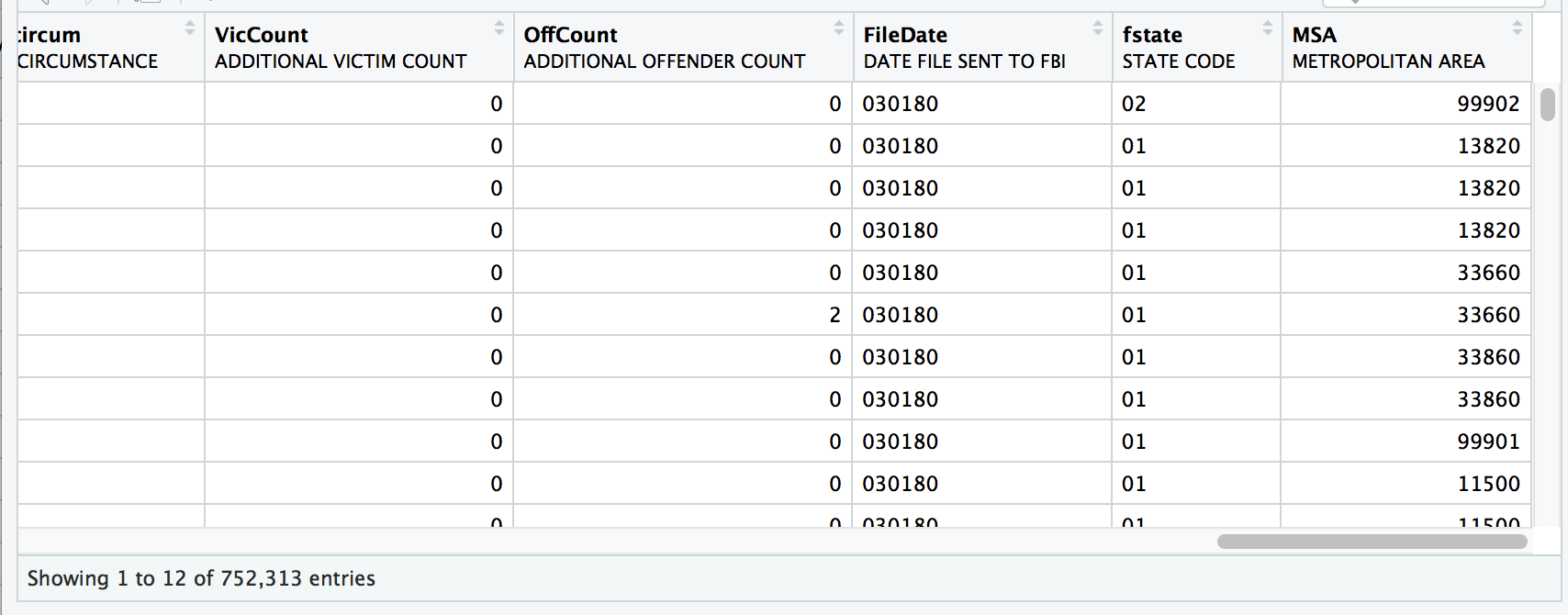

Can you spot the difference?

The data_labels dataframe has the states and metropolitan area columns in the far right spelled out.

The data_only dataframe has states and metropolitan area columns represented as numbers.

This is a big deal because we need both sets of data for our analysis later on.

These are duplicate data frames but sometimes there’s a sort of mirror to the data in the other one.

Combine data frames

This is what we need to do.

Bring in the dplyr package
Rename the columns that are duplicated but have different data
Drop the columns in one data set that are duplicated but are the same in the other
Bring them together (join) as one big happy data frame

This is the first time you will be introduced to the concept of joining data sets, which is one of the most powerful and important things you can do in data analysis. We’ll go over it in the next chapter in more detail.

We’ll use the select() function from the dplyr package that lets you pick and rename specific columns.

library(dplyr)

## OK, we're keeping ID, CNTYFIPS, Ori, State, Agency, and AGENCY_A columns
## And we're going to rename the other ones so that we know they're labels

new_labels <- select(data_labels,
               ID, CNTYFIPS, Ori, State, Agency, AGENCY_A,
               Agentype_label=Agentype,
               Source_label=Source,
               Solved_label=Solved,
               Year,
               Month_label=Month,
               Incident, ActionType,
               Homicide_label=Homicide,
               Situation_label=Situation,
               VicAge,
               VicSex_label=VicSex,
               VicRace_label=VicRace,
               VicEthnic, OffAge,
               OffSex_label=OffSex,
               OffRace_label=OffRace,
               OffEthnic,
               Weapon_label=Weapon,
               Relationship_label=Relationship,
               Circumstance_label=Circumstance,
               Subcircum, VicCount, OffCount, FileDate,
               fstate_label=fstate,
               MSA_label=MSA)

## OK, we're dropping ID, CNTYFIPS, Ori, State, Agency, and AGENCY_A columns
## And we're going to rename the other ones so that we know they're specifically values


new_data_only <- select(data_only,
               Agentype_value=Agentype,
               Source_value=Source,
               Solved_value=Solved,
               Month_value=Month,
               Homicide_value=Homicide,
               Situation_value=Situation,
               VicSex_value=VicSex,
               VicRace_value=VicRace,
               OffSex_value=OffSex,
               OffRace_value=OffRace,
               Weapon_value=Weapon,
               Relationship_value=Relationship,
               Circumstance_value=Circumstance,
               fstate_value=fstate,
               MSA_value=MSA)

# cbind() means column binding-- it only works if the number of rows are the same

new_data <- cbind(new_labels, new_data_only)
 
# Now we're going to use the select() function to reorder the columns so labels and values are next to each other

new_data <- select(new_data,
                ID, CNTYFIPS, Ori, State, Agency, AGENCY_A,
                Agentype_label, Agentype_value,
                Source_label, Source_value,
                Solved_label, Solved_value,
                Year,
                Month_label, Month_value,
                Incident, ActionType,
                Homicide_label,Homicide_value,
                Situation_label,Situation_value,
                VicAge,
                VicSex_label,VicSex_value,
                VicRace_label,VicRace_value,
                VicEthnic, OffAge,
                OffSex_label,OffSex_value,
                OffRace_label,OffRace_value,
                OffEthnic,
                Weapon_label,Weapon_value,
                Relationship_label,Relationship_value,
                Circumstance_label,Circumstance_value,
                Subcircum, VicCount, OffCount, FileDate,
                fstate_label,fstate_value,
                MSA_label,MSA_value)

# remove the old data frames because they're huge and we want to free up memory
rm(data_labels)
rm(data_only)
rm(new_labels)
rm(new_data_only)

How’s it look at the end of the data frame now?

View(new_data)

There are now 47 columns total and it looks like the values are next to labels.

Wonderful.

Let’s move on to the next chapter so we can start wrangling this data.